Left truncation with delay

Some delays are only ever recorded above a minimum value. Generation intervals are often defined to exclude same day transmission. Case definitions sometimes require a minimum time between two events before a pair is recorded. In both settings the observed delays are a left truncated sample from the delay distribution of interest.

Write \(L\) for that minimum and \(F\) for the delay distribution. Only delays above \(L\) can enter the sample, so the observed delays follow the conditional distribution \[ F(t \mid T > L) = \frac{F(t) - F(L)}{1 - F(L)}, \qquad t > L . \] Fitting \(F\) directly to such a sample biases the estimate. The model has to explain the missing short delays by shifting the whole distribution.

With right truncation at \(D\) as well, the likelihood renormalises over \([L, D]\) \[ \frac{F(t) - F(L)}{F(D) - F(L)} . \]

The delay_min argument of as_epidist_marginal_model() sets \(L\). It is passed to the primarycensored likelihood as its L argument. delay_min is a duration in the same units as the delay, not a date.

delay_min truncates on the same scale as the response, that is the observed delay between the primary window lower bound and the secondary event. Data should therefore be excluded on the observed delay rather than on the underlying continuous delay.

1 Setup

library(epidist)
library(ggplot2)
library(dplyr)

2 Simulate left truncated data

We simulate an outbreak and a lognormal delay from each primary event. The parameters are chosen so that a large share of the distribution falls below the truncation point.

set.seed(101)

true_meanlog <- 1.0
true_sdlog <- 0.8
delay_min <- 2

obs <- simulate_gillespie(r = 0.2, seed = 101) |>
  simulate_secondary(
    dist = rlnorm,
    meanlog = true_meanlog,
    sdlog = true_sdlog
  )

Roughly this share of the delay distribution lies below the truncation point.

plnorm(delay_min, true_meanlog, true_sdlog)
#> [1] 0.3506501

simulate_dates() adds daily reporting windows and returns date. We then drop the pairs whose observed delay is below delay_min.

obs_trunc <- obs |>
  simulate_dates() |>
  filter(as.numeric(sdate_lwr - pdate_lwr) >= delay_min) |>
  slice_sample(n = 500)

linelist <- as_epidist_linelist_data(obs_trunc)

The observed delays are truncated below delay_min.

ggplot(linelist, aes(x = stime_lwr - ptime_lwr)) +
  geom_histogram(
    aes(y = after_stat(density)),
    binwidth = 1, fill = "#56B4E9", alpha = 0.7
  ) +
  geom_vline(
    xintercept = delay_min, linetype = "dashed", linewidth = 0.8
  ) +
  labs(x = "Observed delay (days)", y = "Density") +
  theme_minimal()

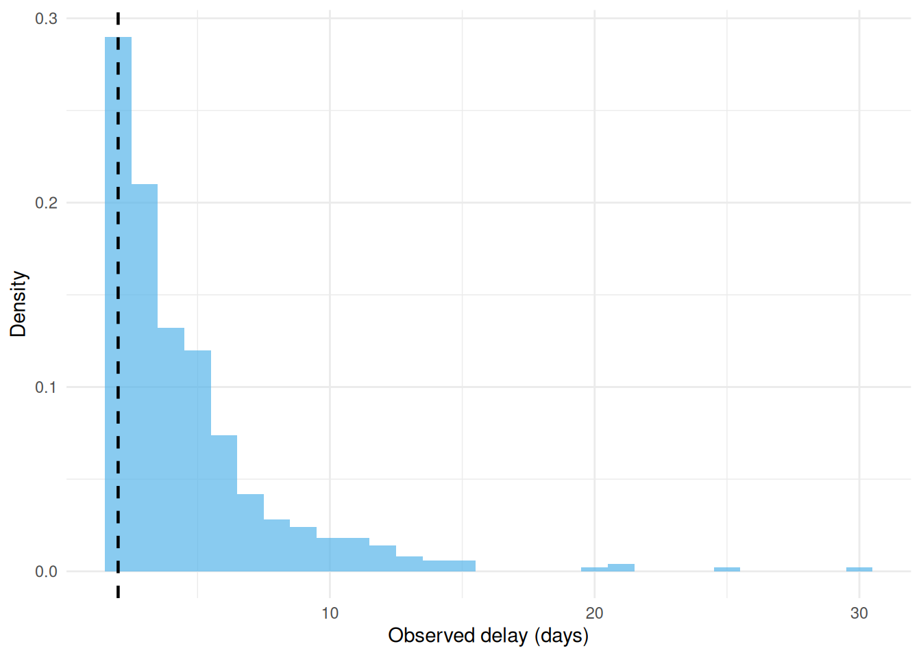
Figure 2.1: Observed delays after left truncation. The dashed line marks the minimum delay.

3 Fit models with and without the adjustment

marginal_no_trunc <- as_epidist_marginal_model(linelist)
marginal_trunc <- as_epidist_marginal_model(linelist, delay_min = delay_min)

A delay_min column already in the data is picked up without the argument. Pass a column name instead of a number when the minimum varies between observations.

linelist$delay_min <- delay_min

identical(
  as_epidist_marginal_model(linelist)$delay_min,
  marginal_trunc$delay_min
)
#> [1] TRUE

delay_min is stored as a column and passed to the likelihood.

marginal_trunc
#> # A tibble: 500 × 19
#>    ptime_lwr ptime_upr stime_lwr stime_upr obs_time  case pdate_lwr  pdate_upr
#>        <dbl>     <dbl>     <dbl>     <dbl>    <dbl> <int> <date>     <date>
#>  1        33        34        38        39       84  7022 2024-02-03 2024-02-04
#>  2        40        41        53        54       84  8003 2024-02-10 2024-02-11
#>  3        13        14        17        18       84  1000 2024-01-14 2024-01-15
#>  4        20        21        28        29       84  2739 2024-01-21 2024-01-22
#>  5        18        19        22        23       84  2301 2024-01-19 2024-01-20
#>  6        26        27        30        31       84  5070 2024-01-27 2024-01-28
#>  7        22        23        26        27       84  3556 2024-01-23 2024-01-24
#>  8        32        33        35        36       84  6810 2024-02-02 2024-02-03
#>  9        11        12        15        16       84   720 2024-01-12 2024-01-13
#> 10        29        30        31        32       84  6148 2024-01-30 2024-01-31
#> # ℹ 490 more rows
#> # ℹ 11 more variables: sdate_lwr <date>, sdate_upr <date>, obs_date <date>,
#> #   pwindow <dbl>, swindow <dbl>, relative_obs_time <dbl>,
#> #   orig_relative_obs_time <dbl>, delay_lwr <dbl>, delay_upr <dbl>, n <dbl>,
#> #   delay_min <dbl>

fit_no_trunc <- epidist(
  marginal_no_trunc,
  chains = 2, cores = 2, refresh = ifelse(interactive(), 250, 0)
)

fit_trunc <- epidist(
  marginal_trunc,
  chains = 2, cores = 2, refresh = ifelse(interactive(), 250, 0)
)

4 Compare parameter estimates

add_delay_parameter_draws() returns posterior draws of the distributional parameters. For the lognormal family mu is the log scale mean and sigma is the log scale standard deviation. We use epidist_strata() to take a single row of the transformed data because there are no covariates here. add_summaries() adds the natural scale mean and standard deviation, and records the family so that the draws can be plotted.

param_draws <- list(
  "No adjustment" = fit_no_trunc,
  "With delay_min" = fit_trunc
) |>
  lapply(\(fit) delay_parameter_draws(fit, newdata = epidist_strata(fit))) |>
  bind_rows(.id = "model") |>
  add_summaries(family = fit_trunc)

true_values <- data.frame(mu = true_meanlog, sigma = true_sdlog) |>
  add_summaries(family = "lognormal") |>
  unlist()

plot(param_draws, by = "model", true_values = true_values)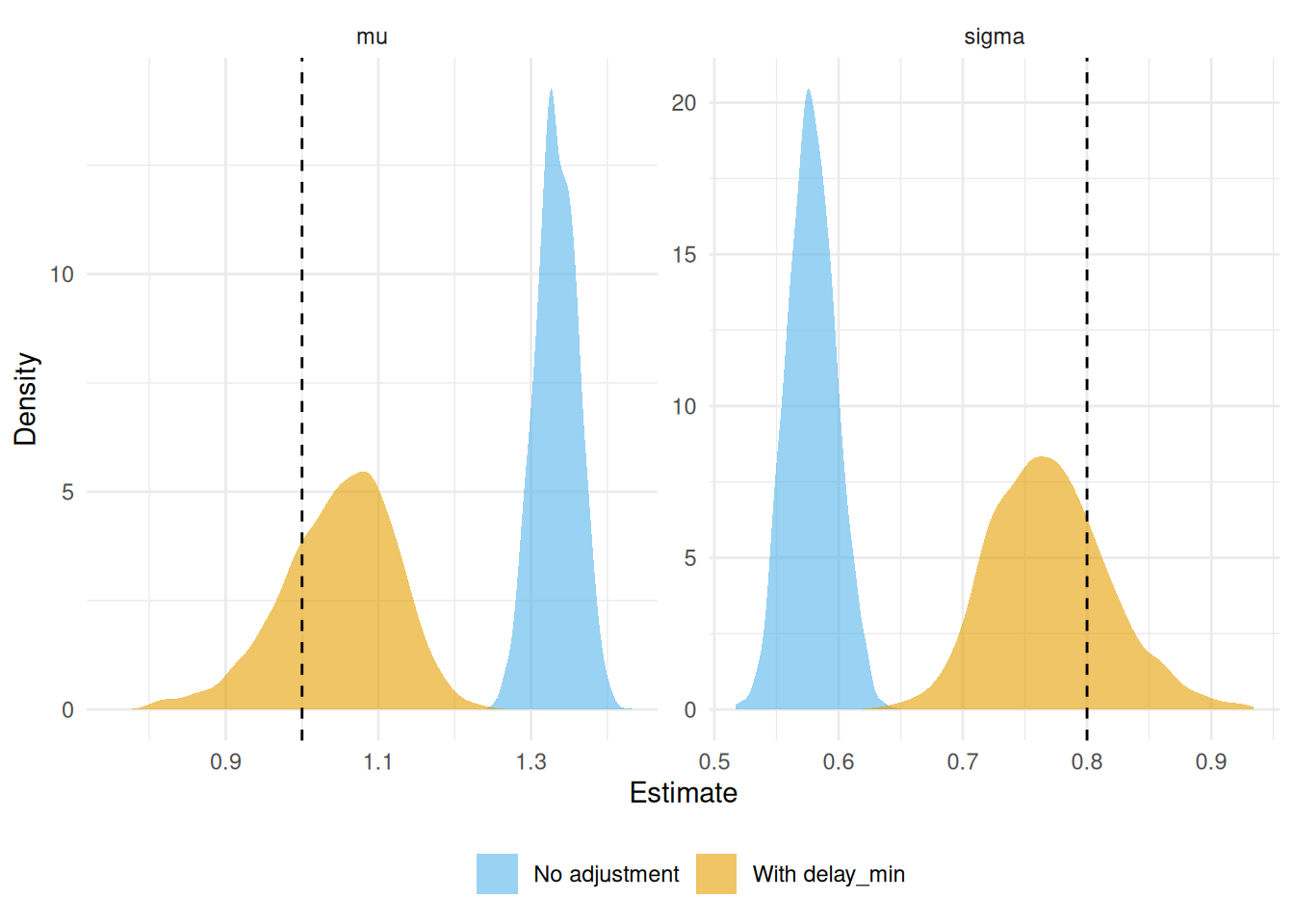

Posterior draws of the lognormal parameters, and of the natural scale mean and standard deviation. Dashed lines are the simulation values. The unadjusted model is biased away from them.

Figure 4.1: Posterior draws of the lognormal parameters, and of the natural scale mean and standard deviation. Dashed lines are the simulation values. The unadjusted model is biased away from them.

The unadjusted model shifts the distribution to the right and understates its spread. The adjusted model recovers the simulation values.

5 Compare the estimated delay distributions

Plotting the same draws with type = "delay" draws the delay distribution each model implies, as the posterior median density with a ribbon between the 5% and 95% quantiles.

plot(param_draws, type = "delay", by = "model") +
  geom_function(
    fun = dlnorm,
    args = list(meanlog = true_meanlog, sdlog = true_sdlog),
    linewidth = 1
  )

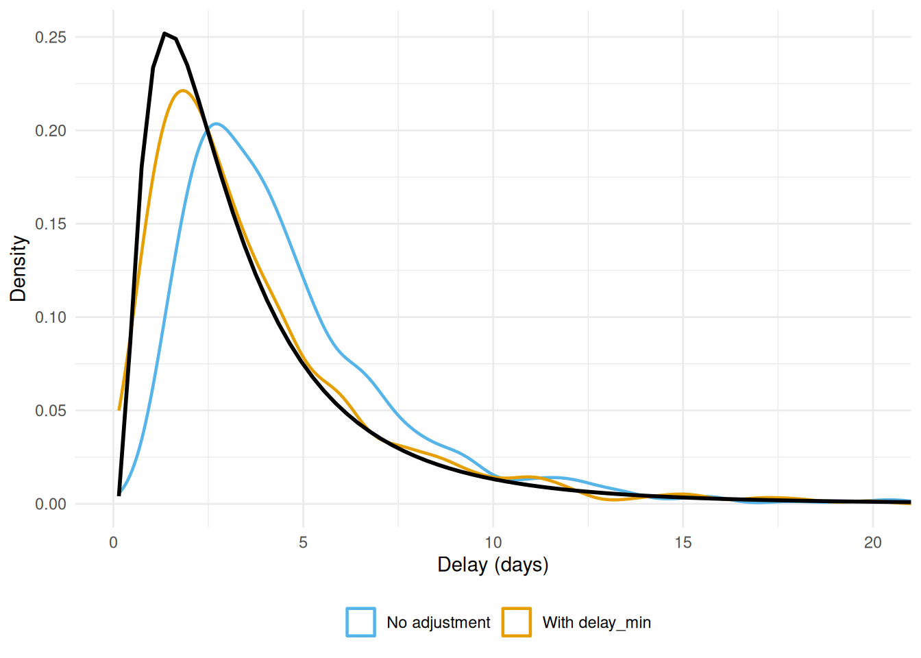
Figure 5.1: Estimated delay distributions against the true lognormal density (black line).

These are the underlying delay distributions rather than the truncated ones, because the distributional parameters do not describe the observation process. Predictions from tidybayes::add_predicted_draws() do the same only when newdata sets delay_min to 0.

6 Summary