Here we provide tips for working with the epidist package, and answers to frequently asked questions.
If you have a question about using the package, please create an issue.
We will endeavour to respond promptly!
Click to expand for code to reproduce the examples in this vignette
library(epidist)
library(brms)
library(dplyr)
library(ggplot2)
library(scales)
library(tidyr)

set.seed(1)

# Define different parameters for each location
meanlog_0 <- 1.6
sdlog_0 <- 0.4
meanlog_1 <- 2.1
sdlog_1 <- 0.6

obs_time <- 25
sample_size <- 200

# Create base data with location assignments
base_data <- simulate_gillespie(seed = 101)
base_data$location <- rbinom(n = nrow(base_data), size = 1, prob = 0.5)

# Create location 0 data
location_0_data <- base_data |>
  filter(location == 0) |>
  simulate_secondary(
    meanlog = meanlog_0,
    sdlog = sdlog_0
  ) |>
  select(case, ptime, delay, stime, location)

# Create location 1 data
location_1_data <- base_data |>
  filter(location == 1) |>
  simulate_secondary(
    meanlog = meanlog_1,
    sdlog = sdlog_1
  ) |>
  select(case, ptime, delay, stime, location)

# Combine datasets
obs_cens_trunc_samp <- bind_rows(location_0_data, location_1_data) |>
  mutate(
    ptime_lwr = floor(.data$ptime),
    ptime_upr = .data$ptime_lwr + 1,
    stime_lwr = floor(.data$stime),
    stime_upr = .data$stime_lwr + 1,
    obs_time = obs_time
  ) |>
  filter(.data$stime_upr <= .data$obs_time) |>
  slice_sample(n = sample_size, replace = FALSE)

linelist_data <- as_epidist_linelist_data(
  obs_cens_trunc_samp$ptime_lwr,
  obs_cens_trunc_samp$ptime_upr,
  obs_cens_trunc_samp$stime_lwr,
  obs_cens_trunc_samp$stime_upr,
  obs_time = obs_cens_trunc_samp$obs_time,
  covariates = data.frame(location = obs_cens_trunc_samp$location)
)
data <- as_epidist_marginal_model(linelist_data)

fit <- epidist(
  data,
  formula = mu ~ 1,
  seed = 1,
  chains = 2,
  cores = 2,
  refresh = ifelse(interactive(), 250, 0),
  iter = 1000,
  backend = "cmdstanr"
)

fit_location <- epidist(
  data,
  formula = bf(mu ~ location, sigma ~ location),
  seed = 1,
  chains = 2,
  cores = 2,
  refresh = ifelse(interactive(), 250, 0),
  iter = 1000,
  backend = "cmdstanr"
)
Working with posterior samples
The output of a call to epidist is compatible with typical Stan workflows.
We recommend use of the posterior package for working with samples.
Getting a data.frame of posterior samples
The function posterior::as_draws_df() may be used to obtain a dataframe of MCMC draws for specified parameters.
library(posterior)
draws <- as_draws_df(fit, variable = c("Intercept", "Intercept_sigma"))
head(draws)
## # A draws_df: 6 iterations, 1 chains, and 2 variables
## Intercept Intercept_sigma
## 1 1.8 -0.59
## 2 1.8 -0.56
## 3 1.8 -0.49
## 4 1.8 -0.61
## 5 1.9 -0.53
## 6 1.9 -0.52
## # ... hidden reserved variables {'.chain', '.iteration', '.draw'}Using random variables (rvars) for uncertainty propagation
The posterior package also provides the rvar class for working with posterior samples as random variables.
This approach allows you to perform mathematical operations directly with posterior distributions while propagating uncertainty.
library(posterior)
# Convert model parameters to rvars
rv <- as_draws_rvars(fit_location)

# Look at the intercept in rvar form
rv$b_Intercept
## rvar<500,2>[1] mean ± sd:
## [1] 1.6 ± 0.063
# Calculate the mean delay (on natural scale) for each location
mean_delay_loc0 <- exp(rv$b_Intercept + 0.5 * exp(rv$b_sigma_Intercept)^2)
mean_delay_loc1 <- exp(rv$b_Intercept +
  rv$b_location + 0.5 * (exp(rv$b_sigma_Intercept + rv$b_sigma_location))^2)

# Summarize the distributions
summary(mean_delay_loc0)
## # A tibble: 1 × 10
## variable mean median sd mad q5 q95 rhat ess_bulk ess_tail
## <chr> <dbl> <dbl> <dbl> <dbl> <dbl> <dbl> <dbl> <dbl> <dbl>
## 1 mean_delay_loc0 5.54 5.48 0.449 0.389 4.95 6.32 1.00 661. 685.
summary(mean_delay_loc1)## # A tibble: 1 × 10
## variable mean median sd mad q5 q95 rhat ess_bulk ess_tail
## <chr> <dbl> <dbl> <dbl> <dbl> <dbl> <dbl> <dbl> <dbl> <dbl>
## 1 mean_delay_loc1 12.8 11.4 5.45 2.82 8.24 21.4 1.01 208. 197.
# Calculate the difference between locations
delay_diff <- mean_delay_loc1 - mean_delay_loc0
delay_diff
## rvar<500,2>[1] mean ± sd:
## [1] 7.3 ± 5.5For more details, see the posterior package documentation.
How can I assess whether sampling has converged?
The output of a call to epidist is compatible with typical Stan workflows.
We recommend use of the bayesplot package for sampling diagnostic plots.
For example, the function bayesplot::mcmc_trace() can be used to produce traceplots for specified parameters.
library(bayesplot)
mcmc_trace(fit, pars = c("Intercept", "Intercept_sigma"))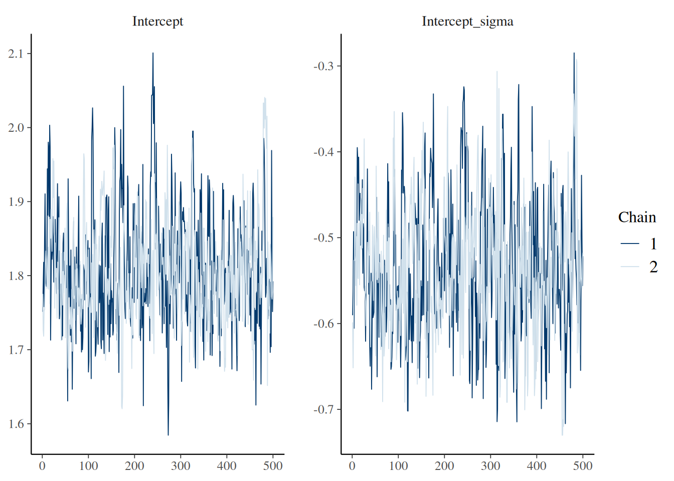
We also provide a function epidist_diagnostics() which can be used to obtain common diagnostics used to assess the quality of a fitted model.
epidist_diagnostics(fit)## # A tibble: 1 × 8
## time samples max_rhat divergent_transitions per_divergent_transitions
## <dbl> <dbl> <dbl> <dbl> <dbl>
## 1 2.51 1000 1.00 0 0
## # ℹ 3 more variables: max_treedepth <dbl>, no_at_max_treedepth <int>,
## # per_at_max_treedepth <dbl>How can I perform posterior predictive checks?
Posterior predictive checks are a useful tool for assessing model fit by comparing observed data to simulated data from the posterior predictive distribution.
brms::pp_check() is a convenient function for this, but it does not automatically handle the aggregated/weighted data structure used by epidist models.
Because brms::pp_check() ignores the weights argument when plotting observed data, passing aggregated data directly will result in an incorrect comparison between observed and predicted distributions.
To use pp_check() correctly with aggregated data, you must first expand the data to an individual-level format (one row per observation) using tidyr::uncount().
Then, pass this expanded data to the newdata argument of pp_check().
# Expand the aggregated data to individual-level data
# Note: We must ensure the weight column 'n' is present but set to 1
data_expanded <- data |>
  tidyr::uncount(weights = n) |>
  mutate(n = 1)

# Run pp_check with the expanded data
pp_check(fit, newdata = data_expanded, ndraws = 100)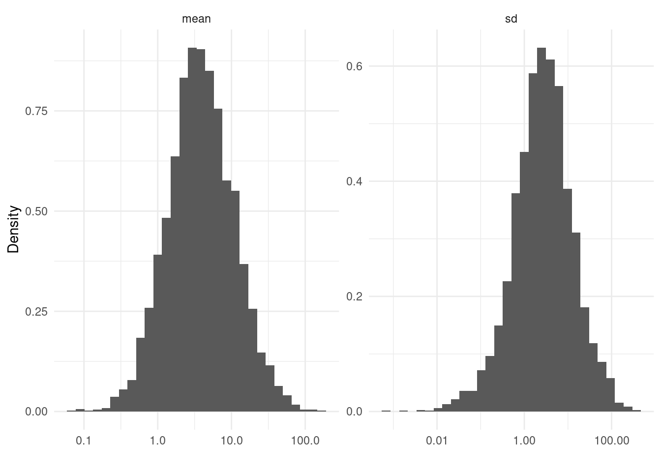
For more advanced custom visualizations, you can also use tidybayes::add_predicted_draws() as demonstrated in the “Advanced features with Ebola data” vignette.
I’d like to run a simulation study
We recommend use of the purrr package for running many epidist models, for example as a part of a simulation study.
We particularly highlight two functions which might be useful:
-
purrr::map()(and other similar functions) for iterating over a list of inputs. -
purrr::safely()which ensures that the function called “always succeeds”. In other words, if there is an error it will be captured and output, rather than ending computation (and potentially disrupting a call topurrr::map()).
For an example use of these functions, have a look at the epidist-paper repository containing the code for Park et al. (2024).
(Note that in that codebase, we use map as a part of a targets pipeline.)
How are the default priors for epidist chosen?
brms provides default priors for all parameters.
However, some of those priors do not make sense in the context of our application.
Instead, we used prior predictive checking to set epidist-specific default priors which produce epidemiological delay distribution mean and standard deviation parameters in a reasonable range.
For example, for the brms::lognormal() latent individual model, we suggest the following prior distributions for the brms mu and sigma intercept parameters:
# Note that we export lognormal() as part of epidist hence no need for brms::
family <- lognormal()

epidist_family <- epidist_family(data, family)
epidist_formula <- epidist_formula(
  data,
  family = epidist_family,
  formula = mu ~ 1
)

# NULL here means no replacing priors from the user!
epidist_prior <- epidist_prior(
  data = data,
  family = family,
  formula = epidist_formula,
  prior = NULL
)

epidist_prior
## prior class coef group resp dpar nlpar lb ub tag source
## student_t(3, 5, 3) Intercept default
## student_t(3, 0, 2.5) Intercept sigma default(Note that the functions epidist_family() and epidist_prior() are mostly for internal use!)
Here are the distributions on the delay distribution mean and standard deviation parameters that these prior distributions imply:
set.seed(1)
fit_ppc <- epidist(
  data = data,
  formula = mu ~ 1,
  family = lognormal(),
  sample_prior = "only",
  seed = 1,
  backend = "cmdstanr"
)
pred <- predict_delay_parameters(fit_ppc)

pred |>
  as.data.frame() |>
  pivot_longer(
    cols = c("mu", "sigma", "mean", "sd"),
    names_to = "parameter",
    values_to = "value"
  ) |>
  filter(parameter %in% c("mean", "sd")) |>
  ggplot(aes(x = value, y = after_stat(density))) +
  geom_histogram() +
  facet_wrap(. ~ parameter, scales = "free") +
  labs(x = "", y = "Density") +
  theme_minimal() +
  scale_x_log10(labels = comma)
## `stat_bin()` using `bins = 30`. Pick better value `binwidth`.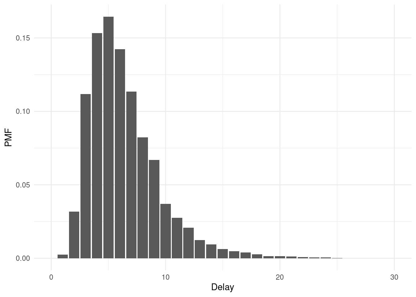
##         1%        10%        25%        50%        75%        90%        99%
## 0.3172760 0.8667011 1.6163277 3.2461963 6.6291746 12.0852973 34.0415723## 1% 10% 25% 50% 75% 90% 99%
## 0.1335500 0.3950604 0.7687361 1.7107506 3.9206460 8.1670947 33.4423697How can I assess how sensitive the fitted posterior distribution is to the prior distribution used?
We recommend use of the priorsense package (Kallioinen et al. 2024) to check how sensitive the posterior distribution is to perturbations of the prior distribution and likelihood using power-scaling analysis:
library(priorsense)
powerscale_plot_dens(fit, variable = c("Intercept", "Intercept_sigma")) +
  theme_minimal()
What do the parameters in my model output correspond to?
The epidist package uses brms to fit models.
This means that the model output will include brms-style names for parameters.
Here, we provide a table giving the correspondence between the distributional parameter names used in brms and those used in standard R functions for some common likelihood families.
| Family |
brms parameter |
R parameter |
|---|---|---|
lognormal() |
mu |
meanlog |
lognormal() |
sigma |
sdlog |
Gamma() |
mu |
shape / scale |
Gamma() |
shape |
shape |
weibull() |
mu |
scale * gamma(1 + 1 / shape) |
weibull() |
shape |
shape |
Note that all families in brms are parameterised with some measure of centrality mu as their first parameter.
This parameter does not necessarily correspond to the mean: hence the provision of a function add_mean_sd() within epidist to add columns containing the natural scale mean and standard deviation to a data.frame of draws.
How can I generate predictions with my fitted epidist model?
It is possible to generate predictions manually by working with samples from the model output.
However this is tricky to do, and so where possible we recommend using the tidybayes package.
In particular, following functions may be useful:
-
tidybayes::add_epred_draws()for predictions of the expected value of a delay. -
tidybayes::add_linpred_draws()for predictions of the delay distributional parameter linear predictors. -
tidybayes::add_predicted_draws()for predictions of the observed delay.
To see these functions demonstrated in a vignette, see “Advanced features with Ebola data”. As a short example, to generate 4000 predictions (equal to the number of draws) of the delay that would be observed with a double censored observation process (in which the primary and secondary censoring windows are both one) then:
##
## Attaching package: 'tidybayes'
## The following objects are masked from 'package:brms':
##
## dstudent_t, pstudent_t, qstudent_t, rstudent_t
draws_pmf <- tibble::tibble(
  relative_obs_time = Inf, pwindow = 1, swindow = 1, delay_upr = NA
) |>
  add_predicted_draws(fit)
## Warning: Found infinite values in the data, which may cause issues for Stan.
ggplot(draws_pmf, aes(x = .prediction)) +
  geom_bar(aes(y = after_stat(count / sum(count)))) +
  labs(x = "Delay", y = "PMF") +
  scale_x_continuous(limits = c(0, 30)) +
  theme_minimal()
## Warning: Removed 6 rows containing non-finite outside the scale range
## (`stat_count()`).## Warning: Removed 1 row containing missing values or values outside the scale range
## (`geom_bar()`).
Importantly, this functionality is only available for epidist models using brms families that have a log_lik_censor method implemented internally in brms. If you are using another family, consider submitting a pull request to implement these methods!
How can I use the marginaleffects package with my fitted epidist model?
The marginaleffects package provides tools for computing and visualising marginal effects, contrasts, and predictions from regression models. It works with epidist models because they are built on top of brms.
For epidist models with covariates, you can use marginaleffects to:
- Compute average marginal effects
- Make comparisons between different covariate values
- Visualise model predictions across the range of covariates
Here’s a simple example using a model that includes location as a covariate:
library(marginaleffects)

# Compare outcomes between location categories (0 and 1)
avg_comparisons(
  fit_location,
  variables = list(location = c(0, 1))
)
##
## Estimate 2.5 % 97.5 %
## 5.86 2.21 20.2
##
## Term: location
## Type: response
## Comparison: 1 - 0For more details on the available functions and their use, see the marginaleffects documentation.
How can I use the cmdstanr backend?
The cmdstanr backend is typically more performant than the default rstan backend.
To use the cmdstanr backend, we first need to install CmdStan (see the README for more details). We can check we have everything we need as follows:
cmdstanr::cmdstan_version()## [1] "2.38.0"