The meta model is experimental. Its interface may still change in future releases.
Systematic reviews of epidemiological delays mostly collect published summaries, such as a mean and standard deviation or a median and interquartile range, rather than individual level data.
Those summaries are often biased, because the studies behind them did not fully adjust for interval censoring or right truncation (Park et al. 2024; Charniga et al. 2024).
The meta model treats the delay as one latent distribution shared by every study.
For each study it applies that study’s estimation procedure to the latent delay, which gives the distribution the study’s summaries estimate.
It then fits each reported summary with a likelihood built from that distribution and the study’s sample size, and fits any individual level data with the likelihood of the marginal model (Abbott et al. 2025).
This covers the most common case, a study that summarised its raw date differences directly, as well as studies that adjusted for some biases.
vignette("model") gives the maths.
Because it is built on brms, formulas, priors and post-processing carry over, so differences between studies are a formula term such as (1 | study).
The ddsynth package also combines individual level data and published summaries, but treats each summary as an unbiased estimate of the delay.
1 What we need from a study
To use a reported summary we need to know how the study estimated it, which reviews rarely record. The meta model needs the following for each study.
-
How the study adjusted for censoring (
cens_adjusted), one of the codes in the table below. -
Whether it adjusted for right truncation (
trunc_adjusted), and if not, the observation time (relative_obs_time) and how collection stopped (trunc_design). For a"cohort"design the observation time is the truncation point on the delay scale. For an"accrual"design, where collection stopped at a calendar date, it is the length of the collection window. -
The censoring windows (
pwindow,swindow), for example 1 for daily reporting or 7 for weekly reporting. -
The sample size (
n) the summary was computed from, or a reported standard error (se). -
The smallest delay it counted (
delay_min), where the study dropped shorter delays, so that its summaries describe a left truncated delay distribution. Defaults to 0, meaning it counted every delay.
cens_adjusted |
The study |
|---|---|
0 |
summarised integer date differences directly, the most common case and the one for summary statistics of raw data |
1 |
used a double interval censored likelihood targeting the continuous delay |
2 |
adjusted only the secondary interval, assuming a uniform delay within it |
3 |
assigned each delay to the centre of the interval it was observed in |
4 |
took the midpoint of the primary event’s window and integrated the secondary interval |
If you cannot tell which of these a study used, state the assumption you are making alongside any results.
See ?as_epidist_estimates_data for the full details.
Where the underlying delays are available and the cutoff that produced them is known, refitting them with the marginal model (vignette("epidist")) is simpler and more reliable than reconstructing what a summary of them means.
The meta model is for the case where the delays cannot be had.
3 Simulating biased published estimates
We simulate an outbreak exactly as in vignette("epidist"), a stochastic epidemic with a lognormal delay between primary (symptom onset) and secondary (case notification) events, both interval censored to a day.
as_epidist_linelist_data() converts the dates to times in days from the first primary event.
We keep the simulated times as well, to work out what each study would have measured.
as_epidist_marginal_model() adds the censoring windows and the bounds of each delay.
Figure 3.1 shows the event windows of the simulated cases.
Code
set.seed(101)
meanlog <- 1.8
sdlog <- 0.5
growth_rate <- 0.2
outbreak_start_date <- as.Date("2024-01-01")

outbreak <- simulate_gillespie(r = growth_rate, seed = 101)
obs <- simulate_secondary(
  outbreak,
  dist = rlnorm, meanlog = meanlog, sdlog = sdlog
)
obs_cens <- simulate_dates(
  obs,
  outbreak_start_date = outbreak_start_date, keep_times = TRUE
)

linelist <- as_epidist_linelist_data(obs_cens)
#> ℹ No observation time column provided, using 2024-04-30 as the observation date (the maximum of the secondary event upper bound).
delays <- as_epidist_marginal_model(linelist)
#> ! Setting 8341 relative observation times (`relative_obs_time`) greater than 74
#>   (2x the maximum delay) to Inf.
#> ℹ This improves model efficiency by reducing the number of unique observation
#>   times in the data.
#> ℹ The impact on model accuracy should be negligible because these relative
#>   observation times are high enough to cause very limited right truncation.
#> ℹ The original relative observation times are available in
#>   `orig_relative_obs_time`.
#> ℹ Raise `obs_time_threshold` to avoid this behaviour.
head(delays)
#> # A tibble: 6 × 22
#>   ptime_lwr ptime_upr stime_lwr stime_upr obs_time  case  ptime delay stime
#>       <dbl>     <dbl>     <dbl>     <dbl>    <dbl> <int>  <dbl> <dbl> <dbl>
#> 1         0         1         5         6      120     1 0.0488  5.59  5.64
#> 2         0         1         9        10      120     2 0.0658  9.76  9.82
#> 3         0         1         8         9      120     3 0.219   7.90  8.12
#> 4         0         1        10        11      120     4 0.250  10.4  10.6
#> 5         0         1         4         5      120     5 0.301   3.98  4.28
#> 6         0         1         9        10      120     6 0.314   9.36  9.68
#> # ℹ 13 more variables: pdate_lwr <date>, pdate_upr <date>, sdate_lwr <date>,
#> #   sdate_upr <date>, obs_date <date>, pwindow <dbl>, swindow <dbl>,
#> #   relative_obs_time <dbl>, orig_relative_obs_time <dbl>, delay_lwr <dbl>,
#> #   delay_upr <dbl>, n <dbl>, delay_min <dbl>
Code
plot_events(linelist)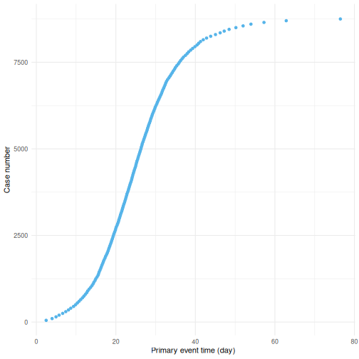
Figure 3.1: The primary and secondary event windows of 200 evenly spaced cases from the simulated outbreak, ordered by primary event time.
Now imagine several studies each analysing this outbreak at a different point in time, reporting integer date differences with no adjustment for right truncation, that is cens_adjusted = 0 and trunc_adjusted = FALSE.
We mimic this by taking cases whose delay is less than a study specific cutoff, since a case with a longer delay would not yet have been observed by that study.
Code
naive_snapshot <- function(cutoff) {
  seen <- delays |>
    filter(.data$delay_upr <= cutoff) |>
    pull(delay_lwr)
  return(tibble(cutoff = cutoff, naive_mean = mean(seen), n = length(seen)))
}

true_mean <- exp(meanlog + sdlog^2 / 2)
bias_illustration <- map(c(4, 6, 8, 12, 16, 25), naive_snapshot) |>
  list_rbind()
Code
ggplot(bias_illustration, aes(x = cutoff, y = naive_mean)) +
  geom_line(col = "#56B4E9") +
  geom_point(col = "#56B4E9", size = 2) +
  geom_hline(yintercept = true_mean, linetype = "dashed") +
  labs(x = "Study cutoff (days)", y = "Naive mean delay (days)") +
  theme_minimal()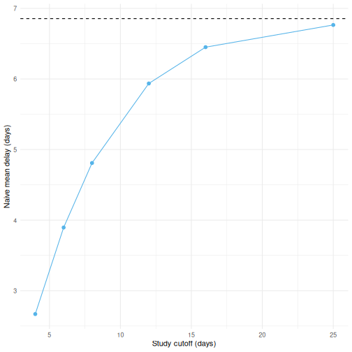
Figure 3.2: The naive mean delay from a snapshot taken with a given cutoff (points), compared to the true mean delay (dashed line). Studies analysing the outbreak earlier see a more heavily right truncated, and so more biased, sample of delays.
Real reviews collect studies that differ in how they measured delays and in what they chose to report.
We build ten such studies from the same line list with simulate_study(), which works out which cases a study would have seen and what it would have measured from them.
Each row of the design below is one study.
Two of them report a mean and standard deviation with the covariance between the two, one adjusted for both biases and one adjusted for neither.
Click to expand for the study designs and the code to build the table
Code
set.seed(2)

# A study that stopped at a calendar date needs the growth rate of primary
# events over its collection window. The simulated outbreak grows more slowly
# than its rate parameter once it starts to deplete susceptibles, so we take
# the realised rate rather than the one we simulated with.
primary_counts <- as_tibble(delays) |>
  filter(.data$ptime_lwr < 20) |>
  count(day = .data$ptime_lwr)
accrual_growth_rate <- coef(
  glm(n ~ day, family = poisson, data = primary_counts)
)[["day"]]

study_designs <- tribble(
  ~study,            ~report,        ~probs,             ~cens_adjusted,
  "naive cohort",    "moments",      NA,                 0,
  "naive IQR",       "quantiles",    c(0.25, 0.5, 0.75), 0,
  "calendar stop",   "quantiles",    c(0.2, 0.5, 0.8),   0,
  "uniform window",  "moments",      NA,                 2,
  "midpoint",        "quantiles",    c(0.3, 0.6, 0.9),   3,
  "adjusted (MVN)",  "multivariate", NA,                 1,
  "naive (MVN)",     "multivariate", NA,                 0,
  "delays over 2d",  "moments",      NA,                 0,
  "mean and se",     "mean_se",      NA,                 0,
  "midpoint window", "moments",      NA,                 4
) |>
  mutate(
    trunc_adjusted = c(
      FALSE, FALSE, FALSE, FALSE, FALSE, TRUE, FALSE, FALSE, FALSE, FALSE
    ),
    relative_obs_time = c(12, 16, 20, 25, 30, Inf, 14, 18, 22, 26),
    trunc_design = c(
      "cohort", "cohort", "accrual", "cohort", "cohort", "cohort",
      "cohort", "cohort", "cohort", "cohort"
    ),
    delay_min = c(0, 0, 0, 0, 0, 0, 0, 2, 0, 0),
    growth_rate = c(0, 0, accrual_growth_rate, 0, 0, 0, 0, 0, 0, 0),
    n = c(180, 55, 240, 95, 40, 300, 150, 130, 25, 110)
  )

studies_table <- study_designs |>
  transmute(
    Study = study,
    Reports = case_when(
      report == "moments" ~ "mean, sd",
      report == "mean_se" ~ "mean with a standard error",
      report == "multivariate" ~ "mean, sd with their covariance",
      .default = paste0("quantiles at p = ", map_chr(probs, toString))
    ),
    Censoring = case_when(
      cens_adjusted == 0 ~ "0: date differences",
      cens_adjusted == 1 ~ "1: fully adjusted",
      cens_adjusted == 2 ~ "2: uniform window",
      cens_adjusted == 3 ~ "3: midpoint",
      .default = "4: midpoint primary, uniform secondary"
    ),
    Truncation = case_when(
      trunc_adjusted ~ "adjusted",
      trunc_design == "accrual" ~ "calendar stop",
      .default = "cohort cutoff"
    ),
    `Obs time` = relative_obs_time,
    `Min delay` = delay_min,
    N = n
  )
Code
knitr::kable(studies_table, caption = "The ten simulated studies, their estimation procedures and what each reports.")| Study | Reports | Censoring | Truncation | Obs time | Min delay | N |
|---|---|---|---|---|---|---|
| naive cohort | mean, sd | 0: date differences | cohort cutoff | 12 | 0 | 180 |
| naive IQR | quantiles at p = 0.25, 0.5, 0.75 | 0: date differences | cohort cutoff | 16 | 0 | 55 |
| calendar stop | quantiles at p = 0.2, 0.5, 0.8 | 0: date differences | calendar stop | 20 | 0 | 240 |
| uniform window | mean, sd | 2: uniform window | cohort cutoff | 25 | 0 | 95 |
| midpoint | quantiles at p = 0.3, 0.6, 0.9 | 3: midpoint | cohort cutoff | 30 | 0 | 40 |
| adjusted (MVN) | mean, sd with their covariance | 1: fully adjusted | adjusted | Inf | 0 | 300 |
| naive (MVN) | mean, sd with their covariance | 0: date differences | cohort cutoff | 14 | 0 | 150 |
| delays over 2d | mean, sd | 0: date differences | cohort cutoff | 18 | 2 | 130 |
| mean and se | mean with a standard error | 0: date differences | cohort cutoff | 22 | 0 | 25 |
| midpoint window | mean, sd | 4: midpoint primary, uniform secondary | cohort cutoff | 26 | 0 | 110 |
simulate_study() takes the line list and the design of one study, so purrr::pmap() builds them one at a time from the rows of the design.
as_epidist_estimates_data() takes the list and combines them.
The same pattern works for a review, with one function that converts a row of the review to the summaries and metadata of a study.
Code
biased_estimates <- study_designs |>
  pmap(simulate_study, data = linelist, max_delay = 60) |>
  as_epidist_estimates_data()
#> ! "naive IQR" (row 3), "calendar stop" (row 6), and "midpoint" (row 11) report
#>   quantiles less than ten days above their smallest counted delay. Quantiles
#>   rounded to whole days that close to the origin carry a bias that a larger
#>   sample does not shrink.
#> ℹ See the Checks section of `?as_epidist_estimates_data`.
biased_estimates
#> # A tibble: 22 × 17
#>    study         type  value    se     n     p pwindow swindow relative_obs_time
#>    <chr>         <chr> <dbl> <dbl> <dbl> <dbl>   <dbl>   <dbl>             <dbl>
#>  1 naive cohort  mean   6.27    NA   180 NA          1       1                12
#>  2 naive cohort  sd     2.50    NA   180 NA          1       1                12
#>  3 naive IQR     quan…  4       NA    55  0.25       1       1                16
#>  4 naive IQR     quan…  6       NA    55  0.5        1       1                16
#>  5 naive IQR     quan…  9       NA    55  0.75       1       1                16
#>  6 calendar stop quan…  3       NA   240  0.2        1       1                20
#>  7 calendar stop quan…  5       NA   240  0.5        1       1                20
#>  8 calendar stop quan…  7       NA   240  0.8        1       1                20
#>  9 uniform wind… mean   6.99    NA    95 NA          1       1                25
#> 10 uniform wind… sd     3.79    NA    95 NA          1       1                25
#> # ℹ 12 more rows
#> # ℹ 8 more variables: trunc_adjusted <lgl>, trunc_design <chr>,
#> #   cens_adjusted <int>, delay_min <dbl>, growth_rate <dbl>,
#> #   growth_rate_sd <dbl>, max_delay <dbl>, mvn_id <chr>
max_delay sets how far the grid behind the implied summaries extends for a study that adjusted for right truncation, since nothing else bounds its delays.
The default suits most delays, so raise it only for a delay with a long tail.
We set it here, and simulate_study() passes it on to as_epidist_estimates_data(), where ?as_epidist_estimates_data.data.frame gives the default.
4 Fitting and comparing models
4.1 A bias-adjusted fit to the summaries alone
We convert the estimates to an epidist_meta_model object and fit it, exactly as we would fit any other epidist model.
Code
meta_summary_only <- as_epidist_meta_model(estimates = biased_estimates)Code
fit_meta_summary <- epidist(
  data = meta_summary_only,
  chains = 2, cores = 2, iter = 1000,
  refresh = ifelse(interactive(), 250, 0),
  seed = 1,
  backend = "cmdstanr"
)
Code
summary(fit_meta_summary)
#>  Family: meta_lognormal
#>   Links: mu = identity; sigma = log
#> Formula: delay_lwr | weights(n) + vint(obs_type, study_n, trunc_adjusted, cens_adjusted, trunc_design, group_start, group_len, chol_start, n_quad, growth_known) + vreal(relative_obs_time, pwindow, swindow, delay_upr, delay_min, report_se, quantile_p, growth_rate) ~ 1
#>          sigma ~ 1
#>    Data: transformed_data (Number of observations: 10)
#>   Draws: 2 chains, each with iter = 1000; warmup = 500; thin = 1;
#>          total post-warmup draws = 1000
#>
#> Regression Coefficients:
#>                 Estimate Est.Error l-95% CI u-95% CI Rhat Bulk_ESS Tail_ESS
#> Intercept           1.82      0.02     1.79     1.85 1.00      915      765
#> sigma_Intercept    -0.74      0.02    -0.78    -0.69 1.00      774      619
#>
#> Draws were sampled using sample(hmc). For each parameter, Bulk_ESS
#> and Tail_ESS are effective sample size measures, and Rhat is the potential
#> scale reduction factor on split chains (at convergence, Rhat = 1).
summary() reports sigma on its log link scale.
delay_parameter_draws() puts both parameters back on the scale the simulation used, and tidybayes::median_qi() summarises the draws.
Code
delay_parameter_draws(fit_meta_summary) |>
  ungroup() |>
  pivot_longer(c("mu", "sigma"), names_to = "parameter") |>
  group_by(.data$parameter) |>
  median_qi(value)
#> # A tibble: 2 × 7
#>   parameter value .lower .upper .width .point .interval
#>   <chr>     <dbl>  <dbl>  <dbl>  <dbl> <chr>  <chr>
#> 1 mu        1.82   1.79   1.85    0.95 median qi
#> 2 sigma     0.477  0.458  0.499   0.95 median qi
Even though every study is individually biased, the meta model recovers the simulated log mean of 1.8 and log standard deviation of 0.5 closely.
4.2 Allowing studies to differ
These ten studies measured one outbreak, so a single mu and sigma is the right model for them.
A real review pools studies of different outbreaks, and some of its metadata will be wrong.
A study level random effect on both parameters, (1 | study), lets each study depart from the population value.
The between study standard deviations get normal(0, 0.25) priors rather than the wide brms default.
init = 0.5 narrows where the chains start, because the default can start a study’s sigma where the model is not finite.
Code
fit_meta_summary_study <- epidist(
  data = meta_summary_only,
  formula = bf(mu ~ 1 + (1 | study), sigma ~ 1 + (1 | study)),
  prior = prior(normal(0, 0.25), class = "sd") +
    prior(normal(0, 0.25), class = "sd", dpar = "sigma"),
  init = 0.5,
  chains = 2, cores = 2, iter = 1000,
  refresh = ifelse(interactive(), 250, 0),
  seed = 1,
  backend = "cmdstanr"
)
Code
fit_meta_summary_study
#>  Family: meta_lognormal
#>   Links: mu = identity; sigma = log
#> Formula: delay_lwr | weights(n) + vint(obs_type, study_n, trunc_adjusted, cens_adjusted, trunc_design, group_start, group_len, chol_start, n_quad, growth_known) + vreal(relative_obs_time, pwindow, swindow, delay_upr, delay_min, report_se, quantile_p, growth_rate) ~ (1 | study)
#>          sigma ~ 1 + (1 | study)
#>    Data: transformed_data (Number of observations: 10)
#>   Draws: 2 chains, each with iter = 1000; warmup = 500; thin = 1;
#>          total post-warmup draws = 1000
#>
#> Multilevel Hyperparameters:
#> ~study (Number of levels: 10)
#>                     Estimate Est.Error l-95% CI u-95% CI Rhat Bulk_ESS Tail_ESS
#> sd(Intercept)           0.03      0.02     0.00     0.09 1.02      220      494
#> sd(sigma_Intercept)     0.08      0.05     0.00     0.21 1.00      297      444
#>
#> Regression Coefficients:
#>                 Estimate Est.Error l-95% CI u-95% CI Rhat Bulk_ESS Tail_ESS
#> Intercept           1.82      0.02     1.78     1.86 1.00      868      676
#> sigma_Intercept    -0.72      0.04    -0.81    -0.62 1.00      644      583
#>
#> Draws were sampled using sample(hmc). For each parameter, Bulk_ESS
#> and Tail_ESS are effective sample size measures, and Rhat is the potential
#> scale reduction factor on split chains (at convergence, Rhat = 1).
re_formula = NA switches the study term off, giving the population level delay, which we compare with the fit without the term.
Figure 4.1 shows the delay distribution each fit implies.
Click to expand for code to prepare the study term plot
Code
population <- epidist_newdata(meta_summary_only)
delay_grid <- seq(0, 40, by = 0.25)

lognormal_band <- function(fit, n = 200) {
  draws <- delay_parameter_draws(
    fit, newdata = population, re_formula = NA
  ) |>
    ungroup()
  out <- draws |>
    slice_sample(n = min(n, nrow(draws))) |>
    mutate(curve = row_number()) |>
    reframe(
      x = delay_grid,
      y = dlnorm(delay_grid, meanlog = .data$mu, sdlog = .data$sigma),
      .by = "curve"
    ) |>
    group_by(.data$x) |>
    median_qi(y, .width = 0.9)
  return(out)
}

study_term_band <- list(
  "mu ~ 1" = fit_meta_summary,
  "mu ~ 1 + (1 | study)" = fit_meta_summary_study
) |>
  map(lognormal_band) |>
  list_rbind(names_to = "model")

true_curve <- tibble(
  x = delay_grid, y = dlnorm(delay_grid, meanlog = meanlog, sdlog = sdlog)
)

p_study_term <- ggplot() +
  geom_ribbon(
    data = study_term_band,
    aes(x = x, ymin = .lower, ymax = .upper, fill = model), alpha = 0.25
  ) +
  geom_line(
    data = study_term_band, aes(x = x, y = y, colour = model),
    linewidth = 0.7
  ) +
  geom_line(data = true_curve, aes(x = x, y = y), linetype = "dashed") +
  scale_colour_brewer(palette = "Set2", aesthetics = c("colour", "fill")) +
  labs(x = "Delay (days)", y = "Density", colour = NULL, fill = NULL) +
  theme_minimal() +
  theme(legend.position = "bottom")
Code
p_study_term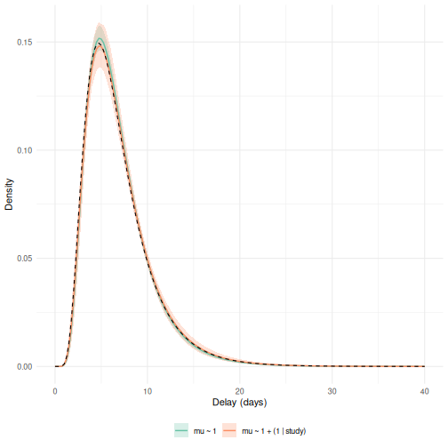
Figure 4.1: The delay distribution implied by the fits with and without a study term. Lines are the posterior median density and bands the 90% interval. The dashed line is the simulated lognormal.
The term widens the band, which is the price of allowing for differences between studies that here do not exist.
4.3 What happens with the wrong metadata
Whether a study corrected for right truncation is the field reviews most often leave out, so we refit the same ten studies with every one of them relabelled as trunc_adjusted = TRUE.
Code
wrong_flags_estimates <- biased_estimates
wrong_flags_estimates$trunc_adjusted <- TRUE
meta_wrong_flags <- as_epidist_meta_model(estimates = wrong_flags_estimates)
Code
fit_meta_wrong_flags <- epidist(
  data = meta_wrong_flags,
  chains = 2, cores = 2, iter = 1000,
  refresh = ifelse(interactive(), 250, 0),
  seed = 1,
  backend = "cmdstanr"
)
Code
summary(fit_meta_wrong_flags)
#>  Family: meta_lognormal
#>   Links: mu = identity; sigma = log
#> Formula: delay_lwr | weights(n) + vint(obs_type, study_n, trunc_adjusted, cens_adjusted, trunc_design, group_start, group_len, chol_start, n_quad, growth_known) + vreal(relative_obs_time, pwindow, swindow, delay_upr, delay_min, report_se, quantile_p, growth_rate) ~ 1
#>          sigma ~ 1
#>    Data: transformed_data (Number of observations: 10)
#>   Draws: 2 chains, each with iter = 1000; warmup = 500; thin = 1;
#>          total post-warmup draws = 1000
#>
#> Regression Coefficients:
#>                 Estimate Est.Error l-95% CI u-95% CI Rhat Bulk_ESS Tail_ESS
#> Intercept           1.76      0.01     1.74     1.79 1.00      597      589
#> sigma_Intercept    -0.83      0.02    -0.87    -0.79 1.00      732      604
#>
#> Draws were sampled using sample(hmc). For each parameter, Bulk_ESS
#> and Tail_ESS are effective sample size measures, and Rhat is the potential
#> scale reduction factor on split chains (at convergence, Rhat = 1).
The model has no way to know the metadata is wrong, so it takes each reported summary as an estimate of the untruncated delay and converges confidently on a mean several percent too short.
4.4 A mixed fit: summaries plus individual records
Now suppose one site also shared its line list.
We add 300 individual records, observed up to day 40, alongside the same ten published summaries.
Individual records keep any study column they arrive with, and are labelled "individual" when they have none, so the study term above extends to line lists from several sites.
Code
individual_data <- linelist |>
  filter(.data$stime_upr <= 40) |>
  mutate(obs_time = 40) |>
  slice_sample(n = 300)

meta_mixed <- as_epidist_meta_model(
  individual_data,
  estimates = biased_estimates
)
#> ! Setting 3 relative observation times (`relative_obs_time`) greater than 38
#>   (2x the maximum delay) to Inf.
#> ℹ This improves model efficiency by reducing the number of unique observation
#>   times in the data.
#> ℹ The impact on model accuracy should be negligible because these relative
#>   observation times are high enough to cause very limited right truncation.
#> ℹ The original relative observation times are available in
#>   `orig_relative_obs_time`.
#> ℹ Raise `obs_time_threshold` to avoid this behaviour.
Code
fit_meta_mixed <- epidist(
  data = meta_mixed,
  chains = 2, cores = 2, iter = 1000,
  refresh = ifelse(interactive(), 250, 0),
  seed = 1,
  backend = "cmdstanr"
)
Code
summary(fit_meta_mixed)
#>  Family: meta_lognormal
#>   Links: mu = identity; sigma = log
#> Formula: delay_lwr | weights(n) + vint(obs_type, study_n, trunc_adjusted, cens_adjusted, trunc_design, group_start, group_len, chol_start, n_quad, growth_known) + vreal(relative_obs_time, pwindow, swindow, delay_upr, delay_min, report_se, quantile_p, growth_rate) ~ 1
#>          sigma ~ 1
#>    Data: transformed_data (Number of observations: 192)
#>   Draws: 2 chains, each with iter = 1000; warmup = 500; thin = 1;
#>          total post-warmup draws = 1000
#>
#> Regression Coefficients:
#>                 Estimate Est.Error l-95% CI u-95% CI Rhat Bulk_ESS Tail_ESS
#> Intercept           1.82      0.01     1.79     1.84 1.00      975      632
#> sigma_Intercept    -0.73      0.02    -0.76    -0.69 1.00      943      541
#>
#> Draws were sampled using sample(hmc). For each parameter, Bulk_ESS
#> and Tail_ESS are effective sample size measures, and Rhat is the potential
#> scale reduction factor on split chains (at convergence, Rhat = 1).
4.5 Reference: the marginal model on the full line list
As a reference, we fit the marginal model (vignette("epidist")) to the whole, effectively untruncated, line list.
This is what we would recover with access to every underlying delay rather than to published summaries.
The marginal model groups identical rows, so the whole line list costs little more to fit than a sample of it.
Code
fit_reference <- epidist(
  data = delays,
  chains = 2, cores = 2, iter = 1000,
  refresh = ifelse(interactive(), 250, 0),
  seed = 1,
  backend = "cmdstanr"
)
4.6 Comparing the fits
Click to expand for code to prepare the comparison plot
Code
predicted_parameters <- list(
  "adjusted (summary only)" = fit_meta_summary,
  "adjusted (study term)" = fit_meta_summary_study,
  "truncation ignored" = fit_meta_wrong_flags,
  mixed = fit_meta_mixed
) |>
  map(delay_summary_draws, newdata = population, re_formula = NA) |>
  c(list("reference (marginal)" = delay_summary_draws(fit_reference))) |>
  map(ungroup) |>
  list_rbind(names_to = "model") |>
  mutate(model = factor(
    model,
    levels = c(
      "truncation ignored", "adjusted (summary only)",
      "adjusted (study term)", "mixed", "reference (marginal)"
    )
  ))

true_sd <- true_mean * sqrt(exp(sdlog^2) - 1)
true_params <- tibble(
  parameter = c("mu", "sigma", "mean", "sd"),
  value = c(meanlog, sdlog, true_mean, true_sd)
)

p_compare <- predicted_parameters |>
  pivot_longer(
    cols = c(mu, sigma, mean, sd),
    names_to = "parameter", values_to = "value"
  ) |>
  ggplot() +
  geom_density(aes(x = value, fill = model), alpha = 0.5) +
  geom_vline(
    data = true_params, aes(xintercept = value),
    linetype = "dashed", linewidth = 1
  ) +
  facet_wrap(~parameter, scales = "free") +
  scale_fill_brewer(palette = "Set2") +
  labs(x = "", y = "", fill = NULL) +
  guides(fill = guide_legend(nrow = 2)) +
  theme_minimal() +
  theme(legend.position = "bottom")
Code
p_compare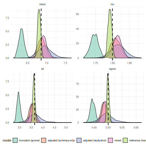
Figure 4.2: Posterior draws of the delay distribution parameters from the five fits, compared to the true values used in the simulation (dashed lines). The bias-adjusted, mixed, and reference fits agree closely with the truth. The fit told that every study had adjusted for right truncation does not.
5 Real world estimates from epireview
epireview (Naidoo et al. 2025) collates published parameter estimates gathered by the Pathogen Epidemiology Review Group. It is not on CRAN, and so we install it from the mrc-ide r-universe.
We use the onset to death delay from the Ebola data.
Code
ebola_params <- as_tibble(suppressMessages(load_epidata("ebola"))$params)
ebola_params
#> # A tibble: 1,225 × 78
#>    id     parameter_data_id covidence_id pathogen parameter_type parameter_value
#>    <chr>  <chr>                    <int> <chr>    <chr>                    <dbl>
#>  1 b6168… 6f5cb18602d0dfec…           30 Ebola v… Human delay -…           NA
#>  2 b6168… b5af335082c4306f…           30 Ebola v… Reproduction …           NA
#>  3 b6168… 55766cedfbf75a9c…           30 Ebola v… Human delay -…           NA
#>  4 0a142… 3ae1f6b55d0f1cc5…           41 Ebola v… Human delay -…            9.2
#>  5 0a142… 22dc037c9e54b6fa…           41 Ebola v… Severity - ca…           60
#>  6 0a142… f0a0191af0663265…           41 Ebola v… Human delay -…            5.8
#>  7 0a142… a83683d0b55750df…           41 Ebola v… Human delay -…           10.6
#>  8 0a142… e8f4a1705568196f…           41 Ebola v… Risk factors             NA
#>  9 67ddf… 5a0a4b5bc6b84974…           45 Ebola v… Severity - ca…           63
#> 10 67ddf… d6d1c36e511e050b…           45 Ebola v… Reproduction …            1.73
#> # ℹ 1,215 more rows
#> # ℹ 72 more variables: exponent <int>, parameter_unit <chr>,
#> #   parameter_lower_bound <dbl>, parameter_upper_bound <dbl>,
#> #   parameter_value_type <chr>, parameter_uncertainty_single_value <dbl>,
#> #   parameter_uncertainty_singe_type <chr>,
#> #   parameter_uncertainty_lower_value <dbl>,
#> #   parameter_uncertainty_upper_value <dbl>, …
epireview records one value per estimate with its type, so we keep the means and medians reported in days with no scaling exponent, and drop inverse rates.
Code
onset_to_death <- ebola_params |>
  filter(
    .data$parameter_type_short == "delay_onset_to_death",
    !is.na(.data$parameter_value),
    !is.na(.data$population_sample_size),
    .data$parameter_value_type %in% c("Mean", "Median"),
    .data$parameter_unit == "Days",
    .data$exponent == 0,
    !.data$inverse_param
  )

shown <- c(
  "article_label", "parameter_value_type", "parameter_value",
  "parameter_unit", "exponent", "inverse_param", "population_sample_size"
)
select(onset_to_death, all_of(shown))
#> # A tibble: 29 × 7
#>    article_label    parameter_value_type parameter_value parameter_unit exponent
#>    <chr>            <chr>                          <dbl> <chr>             <int>
#>  1 Xu 2016          Mean                            8.6  Days                  0
#>  2 Uyeki 2016       Median                         14    Days                  0
#>  3 Senga 2016 (1)   Mean                           11.1  Days                  0
#>  4 Schieffelin 2014 Mean                            9.79 Days                  0
#>  5 Nanclares 2016   Median                          9    Days                  0
#>  6 Qureshi 2015     Mean                            8.9  Days                  0
#>  7 Mupapa 1999      Mean                            8    Days                  0
#>  8 Muoghalu 2017    Mean                            6.7  Days                  0
#>  9 Li 2016 (a)      Median                          4    Days                  0
#> 10 Rosello 2015 (1) Mean                            9.47 Days                  0
#> # ℹ 19 more rows
#> # ℹ 2 more variables: inverse_param <lgl>, population_sample_size <int>
5.1 Adjusting for the phase of the outbreak
An estimate made while an outbreak is still growing is right truncated and biased towards shorter delays, because the long delays have not yet been observed.
vignette("model") sets out the bias and vignette("epidist") shows the marginal model correcting for it.
Correcting for it here needs the observation time of each study, which epireview does not record.
It does record the phase of the outbreak an estimate was made in, so we adjust for that instead and let the size of the bias be estimated from the studies.
We make the post outbreak studies the reference level. The intercept is then the retrospective delay, and each coefficient is the shift in the other groups.
Code
onset_to_death <- onset_to_death |>
  mutate(
    phase = case_when(
      .data$method_moment_value == "Post outbreak" ~ "post outbreak",
      .data$method_moment_value %in% c("Start outbreak", "Mid outbreak") ~
        "during outbreak",
      .default = "unrecorded"
    ),
    phase = factor(
      .data$phase,
      levels = c("post outbreak", "during outbreak", "unrecorded")
    )
  )
count(onset_to_death, phase)
#> # A tibble: 3 × 2
#>   phase               n
#>   <fct>           <int>
#> 1 post outbreak       7
#> 2 during outbreak     2
#> 3 unrecorded         20
epidist_estimates_epireview() turns each record into the rows as_epidist_estimates_data() expects, such as a mean with its standard deviation or a median with its interquartile range.
epireview does not record how a study adjusted for censoring either, so we assume every study summarised integer date differences (cens_adjusted = 0).
Without observation times every study is treated as adjusted for right truncation, and the phase term stands in.
The metadata argument overrides these assumptions for individual studies, and keep carries the phase covariate onto the rows.
See ?epidist_estimates_epireview for how each kind of record is converted.
Code
ebola_estimates <- epidist_estimates_epireview(
  onset_to_death,
  trunc_adjusted = TRUE,
  relative_obs_time = Inf,
  cens_adjusted = 0,
  keep = "phase"
)
#> ℹ No `pwindow` column supplied, assuming a censoring window of 1 (daily
#>   reporting) for every study.
#> ℹ No `swindow` column supplied, assuming a censoring window of 1 (daily
#>   reporting) for every study.
#> ℹ No max_delay column supplied, using the delay beyond which 1% of the second
#>   moment of a lognormal matched to each study's summaries lies (at least 10 and
#>   at most twenty times the largest reported value, in whole secondary windows)
#>   as the grid cutoff, or five times the largest reported value where nothing
#>   can be matched. Raise it if the delay has a longer tail than that, and lower
#>   it to speed up fitting.
#> ! "Nanclares 2016" (row 7), "Li 2016 (a)" (row 14), "Khan 1999" (row 27),
#>   "Camacho 2014" (row 35), "Baron 1983" (row 36), "Bah 2015" (row 38),
#>   "Miglietta 2019" (row 43), and "Nsio 2019" (row 44) report quantiles less
#>   than ten days above their smallest counted delay. Quantiles rounded to whole
#>   days that close to the origin carry a bias that a larger sample does not
#>   shrink.
#> ! "Muoghalu 2017" (row 13), "Rosello 2015 (2)" (row 18), "Maganga 2014" (row
#>   24), and "Folarin 2016" (row 30) report a standard deviation whose relative
#>   standard error is above 0.25 under the lognormal tail their mean implies. A
#>   sampling error that large is far from normal, so the likelihood of the
#>   standard deviation cannot be trusted.
#> ℹ See the Checks section of `?as_epidist_estimates_data`.
ebola_estimates
#> # A tibble: 45 × 18
#>    study         type  value    se     n     p pwindow swindow relative_obs_time
#>    <chr>         <chr> <dbl> <dbl> <dbl> <dbl>   <dbl>   <dbl>             <dbl>
#>  1 Xu 2016       mean   8.6   NA      76 NA          1       1               Inf
#>  2 Xu 2016       sd     4.8   NA      76 NA          1       1               Inf
#>  3 Uyeki 2016    quan… 14     NA       5  0.5        1       1               Inf
#>  4 Senga 2016 (… mean  11.1   NA      92 NA          1       1               Inf
#>  5 Schieffelin … mean   9.79   0.7    38 NA          1       1               Inf
#>  6 Nanclares 20… quan…  9     NA      25  0.5        1       1               Inf
#>  7 Nanclares 20… quan…  7     NA      25  0.25       1       1               Inf
#>  8 Nanclares 20… quan… 12     NA      25  0.75       1       1               Inf
#>  9 Qureshi 2015  mean   8.9   NA      70 NA          1       1               Inf
#> 10 Qureshi 2015  sd     3.8   NA      70 NA          1       1               Inf
#> # ℹ 35 more rows
#> # ℹ 9 more variables: trunc_adjusted <lgl>, trunc_design <chr>,
#> #   cens_adjusted <int>, delay_min <dbl>, growth_rate <dbl>,
#> #   growth_rate_sd <dbl>, max_delay <dbl>, mvn_id <chr>, phase <fct>
We fit a Gamma, which is the family most of these studies fitted, with a (1 | study) term on both the mean and the shape.
The term allows for real heterogeneity across outbreaks and Ebola species, and for studies whose metadata we have got wrong.
Ebola onset to death is thought to take roughly 7 to 14 days, so the intercept prior is centred on ten days, and a prior on the log shape centred on log(2) covers the spreads reported.
Studies may differ by about a quarter on the log scale, so the between study standard deviations get normal(0, 0.25), and the phase coefficients get normal(0, 0.5) so that two studies cannot move the contrast without limit.
epidist_prior() shows the priors the model will use.
Code
ebola_prior <- prior(normal(log(10), 0.5), class = "Intercept") +
  prior(normal(log(2), 0.5), class = "Intercept", dpar = "shape") +
  prior(normal(0, 0.5), class = "b") +
  prior(normal(0, 0.25), class = "sd") +
  prior(normal(0, 0.25), class = "sd", dpar = "shape")

ebola_meta <- as_epidist_meta_model(estimates = ebola_estimates)
ebola_formula <- bf(mu ~ 1 + phase + (1 | study), shape ~ 1 + (1 | study))
ebola_family <- epidist_family(ebola_meta, family = Gamma(link = "log"))

epidist_prior(
  ebola_meta,
  family = ebola_family,
  formula = epidist_formula(ebola_meta, ebola_family, formula = ebola_formula),
  prior = ebola_prior
)
#>                 prior     class coef group resp  dpar nlpar   lb   ub source
#>  normal(log(10), 0.5) Intercept                             <NA> <NA>   user
#>       normal(0, 0.25)        sd                             <NA> <NA>   user
#>       normal(0, 0.25)        sd                 shape       <NA> <NA>   user
#>   normal(log(2), 0.5) Intercept                 shape       <NA> <NA>   user
#>        normal(0, 0.5)         b                             <NA> <NA>   user
#>   tag
#>  <NA>
#>  <NA>
#>  <NA>
#>  <NA>
#>  <NA>
init = 0.5 is passed for the same reason as above.
Code
fit_ebola <- epidist(
  data = ebola_meta,
  formula = ebola_formula,
  family = Gamma(link = "log"),
  prior = ebola_prior,
  init = 0.5,
  chains = 2, cores = 2, iter = 1000,
  refresh = ifelse(interactive(), 250, 0),
  seed = 1,
  backend = "cmdstanr"
)
Code
summary(fit_ebola)
#>  Family: meta_gamma
#>   Links: mu = log; shape = log
#> Formula: delay_lwr | weights(n) + vint(obs_type, study_n, trunc_adjusted, cens_adjusted, trunc_design, group_start, group_len, chol_start, n_quad, growth_known) + vreal(relative_obs_time, pwindow, swindow, delay_upr, delay_min, report_se, quantile_p, growth_rate) ~ phase + (1 | study)
#>          shape ~ 1 + (1 | study)
#>    Data: transformed_data (Number of observations: 29)
#>   Draws: 2 chains, each with iter = 1000; warmup = 500; thin = 1;
#>          total post-warmup draws = 1000
#>
#> Multilevel Hyperparameters:
#> ~study (Number of levels: 29)
#>                     Estimate Est.Error l-95% CI u-95% CI Rhat Bulk_ESS Tail_ESS
#> sd(Intercept)           0.14      0.03     0.08     0.21 1.01      251      629
#> sd(shape_Intercept)     0.52      0.10     0.35     0.74 1.00      385      623
#>
#> Regression Coefficients:
#>                     Estimate Est.Error l-95% CI u-95% CI Rhat Bulk_ESS Tail_ESS
#> Intercept               2.24      0.06     2.12     2.36 1.00      534      616
#> shape_Intercept         1.27      0.15     0.97     1.58 1.00      487      543
#> phaseduringoutbreak     0.06      0.13    -0.19     0.32 1.01      576      401
#> phaseunrecorded        -0.01      0.07    -0.16     0.13 1.00      569      480
#>
#> Draws were sampled using sample(hmc). For each parameter, Bulk_ESS
#> and Tail_ESS are effective sample size measures, and Rhat is the potential
#> scale reduction factor on split chains (at convergence, Rhat = 1).
These estimates should not be used as they stand.
The estimation approach of every study was assumed rather than checked against its paper, which a publication quality meta analysis would have to do.
Only two studies record having been made during an outbreak, so the phase contrast is weak.
The unrecorded group mixes studies where the field is missing with studies where it is unspecified, so the term absorbs whatever separates the groups, which need not be truncation alone.
See Charniga et al. (2024) for the metadata future studies and reviews should report, and andv-linelist-analysis (the Epuyén Andes virus outbreak) and bdbv-linelist-analysis (the 2012 Isiro Bundibugyo Ebola outbreak) for examples of the checklist in use.
5.2 The population level delay and the size of the phase bias
Switching the (1 | study) term off with re_formula = NA gives the population level delay, the one the studies are estimates of rather than any single study’s own.
We report the Gamma shape and scale alongside the mean and standard deviation they imply.
Code
phase_grid <- epidist_newdata(ebola_meta, phase)

population_draws <- delay_summary_draws(
  fit_ebola, newdata = phase_grid, re_formula = NA
) |>
  ungroup()

population_draws |>
  filter(.data$phase == "post outbreak") |>
  mutate(scale = .data$mean / .data$shape) |>
  pivot_longer(c("shape", "scale", "mean", "sd"), names_to = "parameter") |>
  group_by(.data$parameter) |>
  median_qi(value)
#> # A tibble: 4 × 7
#>   parameter value .lower .upper .width .point .interval
#>   <chr>     <dbl>  <dbl>  <dbl>  <dbl> <chr>  <chr>
#> 1 mean       9.36   8.30  10.6    0.95 median qi
#> 2 scale      2.64   1.90   3.65   0.95 median qi
#> 3 sd         4.96   4.08   5.98   0.95 median qi
#> 4 shape      3.55   2.63   4.88   0.95 median qi
The phase bias is the contrast between each phase and the retrospective reference.
marginaleffects::comparisons() gives it as a ratio of mean delays, and its draws give the posterior probability that estimates made during an outbreak are shorter.
Code
phase_ratio <- marginaleffects::comparisons(
  fit_ebola,
  variables = "phase",
  newdata = filter(phase_grid, .data$phase == "post outbreak"),
  re_formula = NA,
  comparison = "ratio"
)
phase_ratio
#>
#>                         Contrast Estimate 2.5 % 97.5 %
#>  during outbreak / post outbreak    1.064 0.831   1.37
#>  unrecorded / post outbreak         0.988 0.854   1.14
#>
#> Term: phase
#> Type: response

marginaleffects::get_draws(phase_ratio) |>
  summarise(
    `P(shorter)` = mean(.data$draw < 1),
    `P(shorter by over 10%)` = mean(.data$draw < 0.9),
    .by = "contrast"
  )
#>                          contrast P(shorter) P(shorter by over 10%)
#> 1 during outbreak / post outbreak      0.302                  0.095
#> 2      unrecorded / post outbreak      0.571                  0.097
5.3 Does any one study drive the estimate?
epidist_meta_leave_one_out() refits the model once per study with that study removed.
Each refit costs as much as the full fit, so we hold out only the five largest studies, which carry the most weight, and refit with 500 iterations.
We compare the population level delay at the post outbreak reference level.
Code
largest_studies <- ebola_estimates |>
  as.data.frame() |>
  summarise(n = max(.data$n), .by = "study") |>
  slice_max(.data$n, n = 5, with_ties = FALSE) |>
  pull("study")

ebola_leave_one_out <- epidist_meta_leave_one_out(
  fit_ebola,
  newdata = filter(phase_grid, .data$phase == "post outbreak"),
  studies = largest_studies,
  iter = 500,
  refresh = ifelse(interactive(), 250, 0)
)
difference is each refit’s posterior relative to the full fit’s median.
Code
ebola_leave_one_out |>
  select("study", "summary", starts_with("difference"))
#> # A tibble: 10 × 5
#>    study            summary difference difference_lower difference_upper
#>    <chr>            <chr>        <dbl>            <dbl>            <dbl>
#>  1 Faye 2015 (b)    mean       0.00792           -1.11             1.35
#>  2 Faye 2015 (b)    sd         0.0249            -0.812            1.13
#>  3 Aylward 2014     mean      -0.0287            -1.27             1.09
#>  4 Aylward 2014     sd        -0.299             -1.07             0.581
#>  5 Miglietta 2019   mean       0.0566            -1.08             1.24
#>  6 Miglietta 2019   sd        -0.0443            -0.941            0.928
#>  7 Rosello 2015 (1) mean      -0.0238            -1.20             1.41
#>  8 Rosello 2015 (1) sd         0.0115            -0.956            1.20
#>  9 Khan 1999        mean      -0.134             -1.41             1.24
#> 10 Khan 1999        sd        -0.0439            -0.927            1.08
Code
ggplot(ebola_leave_one_out) +
  geom_vline(xintercept = 0, linetype = "dashed") +
  geom_pointrange(
    aes(
      x = difference, xmin = difference_lower, xmax = difference_upper,
      y = study
    )
  ) +
  facet_wrap(vars(summary), scales = "free_x") +
  labs(x = "Difference from the full fit (days)", y = "Study held out") +
  theme_minimal()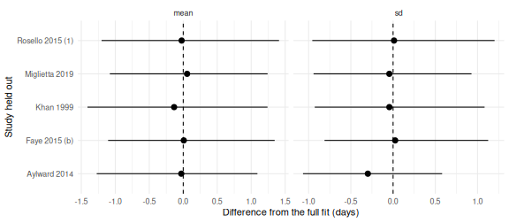
Figure 5.1: Posterior median and 95% interval of the delay mean and standard deviation with each of the five largest studies held out, relative to the full fit’s median.
5.4 Comparing with a modern re-analysis of the same line list
Rosello 2015 (3) is the 2012 Isiro outbreak, and that line list has since been re-analysed in bdbv-linelist-analysis from the individual records, adjusting for double interval censoring.
The outbreak had closed before the line list was published, so the delays are not truncated and the re-analysis is the closest thing to a ground truth for any study we fitted to.
It reports onset to death as a convolution of its fitted onset to admission and admission to death delays, and we match a Gamma to each of 1000 posterior draws of that convolution.
Code
# 1000 draws of the convolution's mean and standard deviation, subsampled
# from the output/posterior_gamma.csv the project releases
bdbv <- read.csv("bdbv-onset-to-death.csv") |>
  mutate(shape = (.data$mean / .data$sd)^2, scale = .data$sd^2 / .data$mean)

isiro_reported <- ebola_estimates |>
  filter(.data$study == "Rosello 2015 (3)") |>
  as.data.frame() |>
  select("type", "value") |>
  pivot_wider(names_from = "type", values_from = "value") |>
  mutate(shape = (.data$mean / .data$sd)^2, scale = .data$sd^2 / .data$mean)

isiro_draws <- epidist_strata(fit_ebola) |>
  filter(.data$study == "Rosello 2015 (3)") |>
  delay_summary_draws(object = fit_ebola) |>
  ungroup()
The mean and standard deviation of the delay, four ways.
Code
interval <- function(draws, source) {
  out <- draws |>
    pivot_longer(c("mean", "sd"), names_to = "parameter") |>
    group_by(.data$parameter) |>
    median_qi(value) |>
    transmute(
      source = source,
      parameter = .data$parameter,
      value = sprintf("%.2f (%.2f, %.2f)", value, .lower, .upper)
    )
  return(out)
}

bind_rows(
  tibble(
    source = "as reported by Rosello 2015 (3)",
    parameter = c("mean", "sd"),
    value = sprintf("%.2f", c(isiro_reported$mean, isiro_reported$sd))
  ),
  interval(isiro_draws, "Rosello 2015 (3), study level"),
  interval(
    filter(population_draws, .data$phase == "post outbreak"),
    "meta model, population level"
  ),
  interval(bdbv, "re-analysis of the line list")
) |>
  pivot_wider(names_from = "parameter", values_from = "value")
#> # A tibble: 4 × 3
#>   source                          mean                sd
#>   <chr>                           <chr>               <chr>
#> 1 as reported by Rosello 2015 (3) 11.37               5.41
#> 2 Rosello 2015 (3), study level   10.65 (9.29, 12.51) 5.22 (4.07, 7.11)
#> 3 meta model, population level    9.36 (8.30, 10.61)  4.96 (4.08, 5.98)
#> 4 re-analysis of the line list    11.76 (9.31, 15.06) 6.57 (4.88, 9.44)
Click to expand for code to prepare the comparison plot
Code
density_band <- function(draws, source, n = 200) {
  out <- draws |>
    slice_sample(n = min(n, nrow(draws))) |>
    mutate(curve = row_number()) |>
    reframe(
      x = delay_grid,
      y = dgamma(delay_grid, shape = .data$shape, scale = .data$scale),
      .by = "curve"
    ) |>
    group_by(.data$x) |>
    median_qi(y) |>
    mutate(source = source)
  return(out)
}

post_outbreak_draws <- population_draws |>
  filter(.data$phase == "post outbreak") |>
  mutate(scale = .data$mean / .data$shape)

comparison_band <- bind_rows(
  density_band(
    mutate(isiro_draws, scale = .data$mean / .data$shape),
    "Rosello 2015 (3), study level"
  ),
  density_band(post_outbreak_draws, "meta model, population level"),
  density_band(bdbv, "re-analysis of the line list")
)

reported_curve <- tibble(
  x = delay_grid,
  y = dgamma(
    delay_grid, shape = isiro_reported$shape, scale = isiro_reported$scale
  )
)

p_bdbv <- ggplot() +
  geom_ribbon(
    data = comparison_band,
    aes(x = x, ymin = .lower, ymax = .upper, fill = source), alpha = 0.25
  ) +
  geom_line(
    data = comparison_band, aes(x = x, y = y, colour = source),
    linewidth = 0.7
  ) +
  geom_line(
    data = reported_curve,
    aes(x = x, y = y, linetype = "as reported by Rosello 2015 (3)"),
    colour = "black", linewidth = 0.7
  ) +
  scale_colour_brewer(palette = "Set2", aesthetics = c("colour", "fill")) +
  scale_linetype_manual(values = "dashed") +
  labs(
    x = "Onset to death delay (days)", y = "Density",
    colour = NULL, fill = NULL, linetype = NULL
  ) +
  theme_minimal() +
  theme(legend.position = "bottom", legend.box = "vertical")
Code
p_bdbv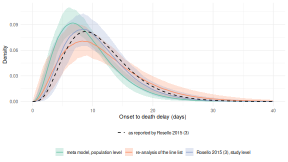
Figure 5.2: The Isiro onset to death delay, four ways. The dashed line is the Gamma reported by Rosello et al. (2015). The bands are 95% posterior intervals of the density from the meta model for the Rosello 2015 (3) study, from the meta model at population level with the (1 | study) term switched off, and from the re-analysis of the same line list.
The study level estimate is shrunk from the reported Gamma towards the population mean by the (1 | study) term on the mean, and keeps the study’s own spread through the term on the shape.
The population level estimate is shorter than the re-analysis.
Most studies carry no usable truncation metadata, so their estimates are taken as adjusted, and the population estimate pools outbreaks that differ.
6 Learning more
- For the marginal and latent models this vignette builds on, see
vignette("epidist"). - For the mathematical detail behind the meta model’s likelihood, see
vignette("model"). - For a real world example fitting the marginal model to individual level Ebola data, see
vignette("ebola").