Using epidist to estimate delay between symptom onset and positive test for an Ebola outbreak in Sierra Leone • epidist

In this vignette, we use the epidist package to analyze line list data from the 2014-2016 outbreak of Ebola in Sierra Leone (World Health Organization 2016). These data were collated by Fang et al. (2016). We provide the data in the epidist package via ?sierra_leone_ebola_data. In analyzing this data, we demonstrate the following features of epidist:

Fitting district-sex stratified partially pooled delay distribution estimates with a lognormal delay distribution.
Post-processing and plotting functionality using the integration of brms functionality with the tidybayes package.

The packages used in this article are:

set.seed(123)

library(epidist)
library(brms)
library(tibble)
library(dplyr)
library(ggplot2)
library(tidybayes)
library(modelr)
library(patchwork)
library(lubridate)
library(cmdstanr) # nolint

For users new to epidist, before reading this article we recommend beginning with the “Getting started with epidist” vignette.

1 Using the cmdstanr backend

As the models explored in this vignette are relatively complex, we recommend using the cmdstanr backend for fitting models as it is typically more performant than the default rstan backend. To use the cmdstanr backend, we first need to install CmdStan (see the README for more details). We can check we have everything we need as follows:

cmdstanr::cmdstan_version()
#> [1] "2.36.0"

2 Data preparation

We begin by loading the Ebola line list data:

data("sierra_leone_ebola_data")

The data has 8358 rows, each corresponding to a unique case report ID (id). The columns of the data are the, age, sex, the dates of Ebola symptom onset and positive sample, and their district and chiefdom.

head(sierra_leone_ebola_data)
#> # A tibble: 6 × 7
#>      id   age sex    date_of_symptom_onset date_of_sample_tested district
#>   <int> <dbl> <chr>  <date>                <date>                <chr>   
#> 1     1    20 Female 2014-05-18            2014-05-23            Kailahun
#> 2     2    42 Female 2014-05-20            2014-05-25            Kailahun
#> 3     3    45 Female 2014-05-20            2014-05-25            Kailahun
#> 4     4    15 Female 2014-05-21            2014-05-26            Kailahun
#> 5     5    19 Female 2014-05-21            2014-05-26            Kailahun
#> 6     6    55 Female 2014-05-21            2014-05-26            Kailahun
#> # ℹ 1 more variable: chiefdom <chr>

fraction <- 5
ndistrict <- length(unique(sierra_leone_ebola_data$district))

Figure 2.1 shows the dates of symptom onset and sample testing for cases across in each district. (In this figure, we filter down to every 5th case in order to avoid overplotting.) We can see that the start time and course of the epidemic varies across districts.

sierra_leone_ebola_data |>
  filter(id %% fraction == 0) |>
  ggplot() +
  geom_segment(
    aes(
      x = date_of_symptom_onset, xend = date_of_sample_tested,
      y = id, yend = id
    ),
    col = "grey"
  ) +
  geom_point(aes(x = date_of_symptom_onset, y = id), col = "#56B4E9") +
  geom_point(aes(x = date_of_sample_tested, y = id), col = "#009E73") +
  facet_wrap(district ~ ., ncol = 2) +
  labs(x = "", y = "Case ID") +
  theme_minimal()

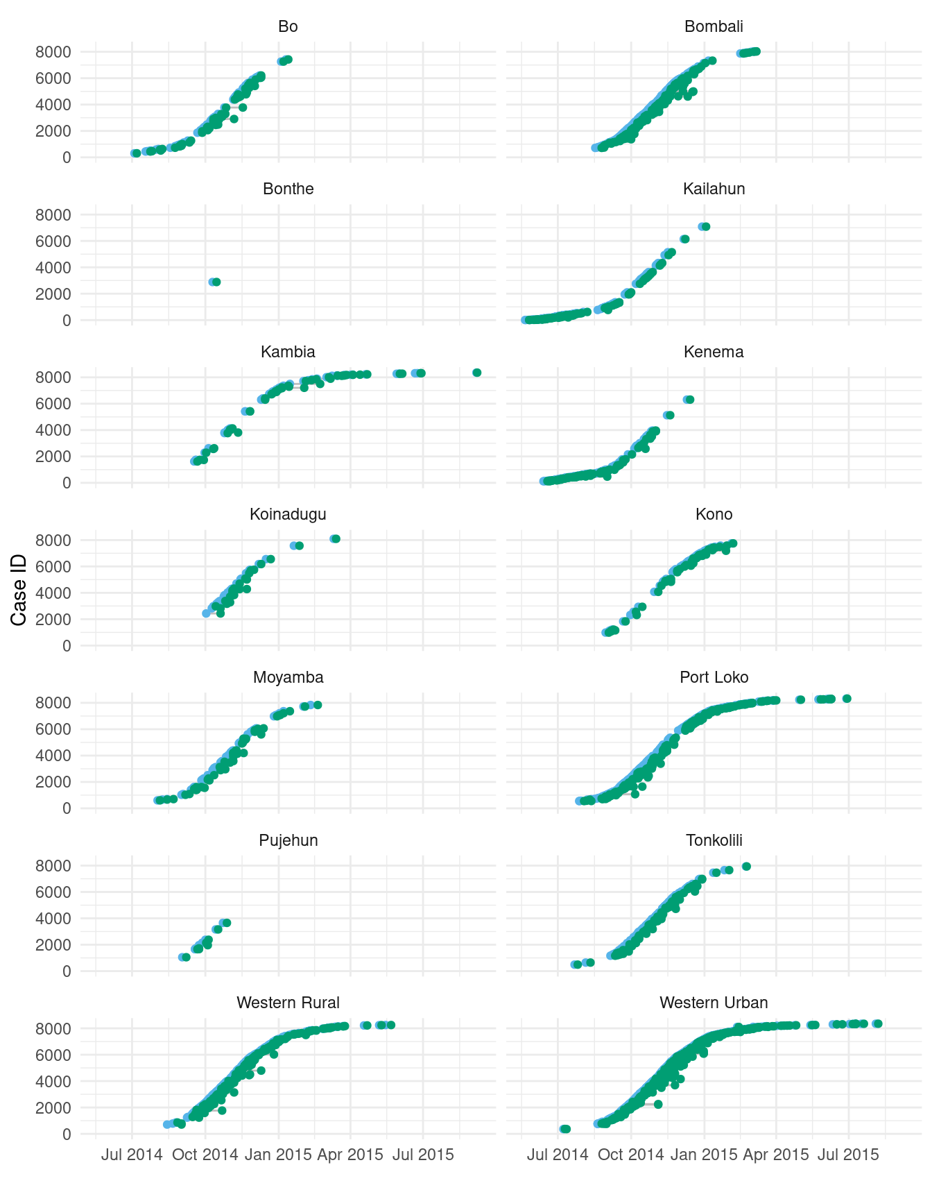
Figure 2.1: Primary and secondary event times for every 5th case, over the 14 districts of Sierra Leone.

3 Fitting sex-district stratified delay distributions

To understand the delay between time of symptom onset and time of sample testing, we fit a range of statistical models using the epidist package. In some models, we vary the parameters of the delay distribution by sex or by district. For the lognormal delay distribution these parameters are the mean and standard deviation of the underlying normal distribution. That is, \(\mu\) and \(\sigma\) such that when \(x \sim \mathcal{N}(\mu, \sigma)\) then \(\exp(x)\) has a lognormal distribution.

3.1 Data preparation

To prepare the data, we begin by selecting the relevant columns:

obs_cens <- sierra_leone_ebola_data |>
  select(id, date_of_symptom_onset, date_of_sample_tested, age, sex, district)

head(obs_cens)
#> # A tibble: 6 × 6
#>      id date_of_symptom_onset date_of_sample_tested   age sex    district
#>   <int> <date>                <date>                <dbl> <chr>  <chr>   
#> 1     1 2014-05-18            2014-05-23               20 Female Kailahun
#> 2     2 2014-05-20            2014-05-25               42 Female Kailahun
#> 3     3 2014-05-20            2014-05-25               45 Female Kailahun
#> 4     4 2014-05-21            2014-05-26               15 Female Kailahun
#> 5     5 2014-05-21            2014-05-26               19 Female Kailahun
#> 6     6 2014-05-21            2014-05-26               55 Female Kailahun

For the time being, we filter the data to only complete cases (i.e. rows of the data which have no missing values¹).

n <- nrow(obs_cens)
obs_cens <- obs_cens[complete.cases(obs_cens), ]
n_complete <- nrow(obs_cens)

To simulate being in the middle of an outbreak we will filter the data to only include cases up to the 31st of January 2015. The marginal model used in this is adjusting for truncation. To check it is working try filtering instead for the date_of_symptom_onset and rerunning.

obs_cens <- obs_cens |>
  filter(date_of_sample_tested <= as.Date("2015-01-31"))

We prepare the data for use with the epidist package by converting the data to an epidist_linelist_data object:

linelist_data <- obs_cens |>
  as_epidist_linelist_data(
    pdate_lwr = "date_of_symptom_onset",
    sdate_lwr = "date_of_sample_tested"
  )

In this call to as_epidist_linelist_data() it has made some assumptions about the data. First, because we did not supply upper bounds for the primary and secondary events (pdate_upr and sdate_upr), it has assumed that the upper bounds are one day after the lower bounds. Second, because we also did not supply an observation time column (obs_date), it has assumed that the observation time is the maximum of the secondary event upper bounds.

3.2 Model fitting

To prepare the data for use with the marginal model, we define the data as being a epidist_marginal_model model object:

obs_prep <- as_epidist_marginal_model(linelist_data, obs_time_threshold = 1)
head(obs_prep)
#> # A tibble: 6 × 21
#>   ptime_lwr ptime_upr stime_lwr stime_upr obs_time    id pdate_lwr  sdate_lwr 
#>       <dbl>     <dbl>     <dbl>     <dbl>    <dbl> <int> <date>     <date>    
#> 1         0         1         5         6      259     1 2014-05-18 2014-05-23
#> 2         2         3         7         8      259     2 2014-05-20 2014-05-25
#> 3         2         3         7         8      259     3 2014-05-20 2014-05-25
#> 4         3         4         8         9      259     4 2014-05-21 2014-05-26
#> 5         3         4         8         9      259     5 2014-05-21 2014-05-26
#> 6         3         4         8         9      259     6 2014-05-21 2014-05-26
#> # ℹ 13 more variables: age <dbl>, sex <chr>, district <chr>, pdate_upr <date>,
#> #   sdate_upr <date>, obs_date <date>, pwindow <dbl>, swindow <dbl>,
#> #   relative_obs_time <dbl>, orig_relative_obs_time <dbl>, delay_lwr <dbl>,
#> #   delay_upr <dbl>, n <dbl>

Now we are ready to fit the marginal model. Note that here we set obs_time_threshold to 1 rather than the default of 2 because we are confident that our data contains the maximum observable delay. If we were not then the default or higher values would be sensible. Try out other models using as_epidist_latent_model() for the latent model (another approach to adjusting for truncation and censoring) and as_epidist_naive_model() for a naive model that doesn’t account for truncation or censoring.

3.2.1 Intercept-only model

We start by fitting a single lognormal distribution to the data. This model assumes that a single distribution describes all delays in the data, regardless of the case’s location, sex, or any other covariates. To do this, we set formula = mu ~ 1 to place an model with only an intercept parameter (i.e. ~ 1 in R formula syntax) on the mu parameter of the lognormal distribution specified using family = lognormal(). (Note that the lognormal distribution has two distributional parameters mu and sigma. As a model is not explicitly placed on sigma, a constant model sigma ~ 1 is assumed.)

fit <- epidist(
  data = obs_prep,
  formula = mu ~ 1,
  family = lognormal(),
  algorithm = "sampling",
  chains = 2,
  cores = 2,
  refresh = ifelse(interactive(), 250, 0),
  seed = 1,
  backend = "cmdstanr"
)
#> Running MCMC with 2 parallel chains...
#> Chain 2 finished in 6.2 seconds.
#> Chain 1 finished in 7.2 seconds.
#> 
#> Both chains finished successfully.
#> Mean chain execution time: 6.7 seconds.
#> Total execution time: 7.4 seconds.

The fit object is a brmsfit object, and has the associated range of methods. See methods(class = "brmsfit") for more details. For example, we may use summary() to view information about the fitted model, including posterior estimates for the regression coefficients:

summary(fit)
#>  Family: marginal_lognormal 
#>   Links: mu = identity; sigma = log 
#> Formula: delay_lwr | weights(n) + vreal(relative_obs_time, pwindow, swindow, delay_upr) ~ 1 
#>          sigma ~ 1
#>    Data: transformed_data (Number of observations: 380) 
#>   Draws: 2 chains, each with iter = 2000; warmup = 1000; thin = 1;
#>          total post-warmup draws = 2000
#> 
#> Regression Coefficients:
#>                 Estimate Est.Error l-95% CI u-95% CI Rhat Bulk_ESS Tail_ESS
#> Intercept           1.65      0.01     1.64     1.67 1.00     1946     1261
#> sigma_Intercept    -0.56      0.01    -0.58    -0.54 1.00     1751     1160
#> 
#> Draws were sampled using sample(hmc). For each parameter, Bulk_ESS
#> and Tail_ESS are effective sample size measures, and Rhat is the potential
#> scale reduction factor on split chains (at convergence, Rhat = 1).

3.2.2 Sex-stratified model

To fit a model which varies the parameters of the fitted lognormal distribution, mu and sigma, by sex we alter the formula specification to include fixed effects for sex ~ 1 + sex as follows:

fit_sex <- epidist(
  data = obs_prep,
  formula = bf(mu ~ 1 + sex, sigma ~ 1 + sex),
  family = lognormal(),
  algorithm = "sampling",
  chains = 2,
  cores = 2,
  refresh = ifelse(interactive(), 250, 0),
  seed = 1,
  backend = "cmdstanr"
)
#> Running MCMC with 2 parallel chains...
#> Chain 2 finished in 14.2 seconds.
#> Chain 1 finished in 14.8 seconds.
#> 
#> Both chains finished successfully.
#> Mean chain execution time: 14.5 seconds.
#> Total execution time: 14.9 seconds.

A summary of the model shows that males tend to have longer delays (the posterior mean of sexMale is 0.04) and greater delay variation (the posterior mean of sigma_sexMale is 0.02). For the sexMale effect, the 95% credible interval is greater than zero, whereas for the sigma_sexMale effect the 95% credible interval includes zero. It is important to note that the estimates represent an average of the observed data, and individual delays between men and women vary significantly.

summary(fit_sex)
#>  Family: marginal_lognormal 
#>   Links: mu = identity; sigma = log 
#> Formula: delay_lwr | weights(n) + vreal(relative_obs_time, pwindow, swindow, delay_upr) ~ sex 
#>          sigma ~ 1 + sex
#>    Data: transformed_data (Number of observations: 584) 
#>   Draws: 2 chains, each with iter = 2000; warmup = 1000; thin = 1;
#>          total post-warmup draws = 2000
#> 
#> Regression Coefficients:
#>                 Estimate Est.Error l-95% CI u-95% CI Rhat Bulk_ESS Tail_ESS
#> Intercept           1.63      0.01     1.61     1.65 1.00     2033     1531
#> sigma_Intercept    -0.58      0.01    -0.60    -0.55 1.00     2072     1530
#> sexMale             0.04      0.01     0.01     0.07 1.00     2283     1568
#> sigma_sexMale       0.02      0.02    -0.02     0.06 1.00     2001     1546
#> 
#> Draws were sampled using sample(hmc). For each parameter, Bulk_ESS
#> and Tail_ESS are effective sample size measures, and Rhat is the potential
#> scale reduction factor on split chains (at convergence, Rhat = 1).

3.2.3 Sex-district stratified model

Finally, we will fit a model which also varies by district. To do this, we will use district level random effects, assumed to be drawn from a shared normal distribution, within the model for both the mu and sigma parameters. These random effects are specified by including (1 | district) in the formulas:

fit_sex_district <- epidist(
  data = obs_prep,
  formula = bf(
    mu ~ 1 + sex + (1 | district),
    sigma ~ 1 + sex + (1 | district)
  ),
  family = lognormal(),
  algorithm = "sampling",
  chains = 2,
  cores = 2,
  iter = 1000,
  refresh = ifelse(interactive(), 250, 0),
  seed = 1,
  backend = "cmdstanr"
)
#> Running MCMC with 2 parallel chains...
#> Chain 2 finished in 203.0 seconds.
#> Chain 1 finished in 220.9 seconds.
#> 
#> Both chains finished successfully.
#> Mean chain execution time: 211.9 seconds.
#> Total execution time: 221.0 seconds.

As this is a longer running model (~ 2 minutes) we have reduced the number of iterations but for real world use cases this may not be sufficient.

For this model, along with looking at the summary(), we may also use the brms::ranef() function to look at the estimates of the random effects:

summary(fit_sex_district)
#>  Family: marginal_lognormal 
#>   Links: mu = identity; sigma = log 
#> Formula: delay_lwr | weights(n) + vreal(relative_obs_time, pwindow, swindow, delay_upr) ~ sex + (1 | district) 
#>          sigma ~ 1 + sex + (1 | district)
#>    Data: transformed_data (Number of observations: 1296) 
#>   Draws: 2 chains, each with iter = 1000; warmup = 500; thin = 1;
#>          total post-warmup draws = 1000
#> 
#> Multilevel Hyperparameters:
#> ~district (Number of levels: 14) 
#>                     Estimate Est.Error l-95% CI u-95% CI Rhat Bulk_ESS Tail_ESS
#> sd(Intercept)           0.16      0.04     0.10     0.24 1.00      258      373
#> sd(sigma_Intercept)     0.20      0.05     0.13     0.33 1.04      165      332
#> 
#> Regression Coefficients:
#>                 Estimate Est.Error l-95% CI u-95% CI Rhat Bulk_ESS Tail_ESS
#> Intercept           1.63      0.04     1.54     1.71 1.01      257      466
#> sigma_Intercept    -0.66      0.06    -0.79    -0.55 1.00      264      411
#> sexMale             0.04      0.01     0.01     0.07 1.00     1312      691
#> sigma_sexMale       0.02      0.02    -0.02     0.06 1.00     1616      761
#> 
#> Draws were sampled using sample(hmc). For each parameter, Bulk_ESS
#> and Tail_ESS are effective sample size measures, and Rhat is the potential
#> scale reduction factor on split chains (at convergence, Rhat = 1).
ranef(fit_sex_district)
#> $district
#> , , Intercept
#> 
#>                    Estimate  Est.Error         Q2.5       Q97.5
#> Bo            -3.838507e-03 0.05347376 -0.110682275  0.10185087
#> Bombali        2.581286e-01 0.04472119  0.174180825  0.34849830
#> Bonthe        -1.862213e-02 0.13306808 -0.299108475  0.24800622
#> Kailahun      -9.955586e-05 0.04513036 -0.091952980  0.08956600
#> Kambia        -5.973642e-02 0.05880347 -0.176033550  0.05695112
#> Kenema        -2.480167e-01 0.05043556 -0.348884675 -0.15341470
#> Koinadugu      1.856984e-01 0.07527595  0.044445255  0.33407015
#> Kono          -7.707571e-02 0.05419185 -0.179583950  0.03888698
#> Moyamba       -7.067646e-03 0.06004876 -0.125565400  0.11777542
#> Port Loko      1.454416e-01 0.04598757  0.055714808  0.23771160
#> Pujehun       -5.130905e-02 0.09275505 -0.230238975  0.13392550
#> Tonkolili      8.347059e-02 0.04697200 -0.008465083  0.17489370
#> Western Rural -2.038493e-02 0.04587658 -0.110987350  0.07276795
#> Western Urban -1.505765e-01 0.04555376 -0.242774150 -0.06006802
#> 
#> , , sigma_Intercept
#> 
#>                  Estimate  Est.Error        Q2.5      Q97.5
#> Bo             0.18896215 0.07296301  0.05330906  0.3352376
#> Bombali       -0.22756598 0.06220791 -0.34967355 -0.0960459
#> Bonthe        -0.13516201 0.20615938 -0.57906983  0.2538547
#> Kailahun      -0.33400693 0.06548897 -0.45963662 -0.1942981
#> Kambia         0.05900935 0.08002008 -0.09201563  0.2221611
#> Kenema         0.11135971 0.06839117 -0.01683754  0.2521803
#> Koinadugu      0.07387654 0.09657278 -0.11703302  0.2542935
#> Kono           0.03210721 0.07086334 -0.09476273  0.1735740
#> Moyamba        0.09484336 0.07423207 -0.04620333  0.2429108
#> Port Loko     -0.02356363 0.06397508 -0.14071705  0.1052845
#> Pujehun       -0.09048644 0.15079205 -0.37209650  0.2205086
#> Tonkolili     -0.15436247 0.06547716 -0.27559662 -0.0215666
#> Western Rural  0.07162684 0.06427340 -0.04773832  0.2033333
#> Western Urban  0.26897389 0.06036981  0.15346425  0.3954492

3.3 Posterior expectations

To go further than summaries of the fitted model, we recommend using the tidybayes package. For example, to obtain the posterior expectation of the delay distribution, under no censoring or truncation, we may use the modelr::data_grid() function in combination with the tidybayes::add_epred_draws() function. The tidybayes::add_epred_draws() function uses the epidist_gen_posterior_predict() function to generate a posterior prediction function for the lognormal() distribution.

In Figure 3.1 we show the posterior expectation of the delay distribution for each of the three fitted models. Figure 3.1B illustrates the higher mean of men as compared with women.

# add dummmy variables
add_marginal_dummy_vars <- function(data) {
  data |>
    mutate(relative_obs_time = NA, pwindow = NA, delay_upr = NA, swindow = NA)
}

epred_draws <- obs_prep |>
  data_grid(NA) |>
  add_marginal_dummy_vars() |>
  add_epred_draws(fit, dpar = TRUE)

epred_base_figure <- epred_draws |>
  ggplot(aes(x = .epred)) +
  stat_halfeye() +
  labs(x = "", y = "", title = "Intercept-only", tag = "A") +
  theme_minimal()

epred_draws_sex <- obs_prep |>
  data_grid(sex) |>
  add_marginal_dummy_vars() |>
  add_epred_draws(fit_sex, dpar = TRUE)

epred_sex_figure <- epred_draws_sex |>
  ggplot(aes(x = .epred, y = sex)) +
  stat_halfeye() +
  labs(x = "", y = "", title = "Sex-stratified", tag = "B") +
  theme_minimal()

epred_draws_sex_district <- obs_prep |>
  data_grid(sex, district) |>
  add_marginal_dummy_vars() |>
  add_epred_draws(fit_sex_district, dpar = TRUE)

epred_sex_district_figure <- epred_draws_sex_district |>
  ggplot(aes(x = .epred, y = district)) +
  stat_pointinterval() +
  facet_grid(. ~ sex) +
  labs(
    x = "Posterior expectation of the delay", y = "",
    title = "Sex-district-stratified", tag = "C"
  ) +
  scale_y_discrete(limits = rev) +
  theme_minimal()

epred_base_figure / epred_sex_figure / epred_sex_district_figure +
  plot_layout(heights = c(1, 1.5, 2.5))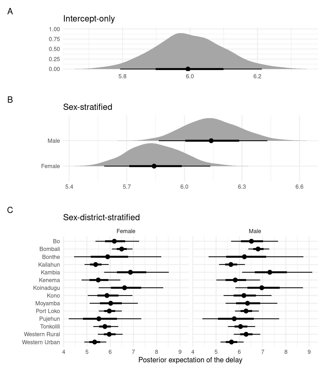

Figure 3.1: The fitted posterior expectations of the delay distribution for each model.

3.4 Linear predictor posteriors

The tidybayes package also allows users to generate draws of the linear predictors for all distributional parameters using tidybayes::add_linpred_draws(). For example, for the mu parameter in the sex-district stratified model (Figure 3.2):

linpred_draws_sex_district <- obs_prep |>
  as.data.frame() |>
  data_grid(sex, district) |>
  add_marginal_dummy_vars() |>
  add_linpred_draws(fit_sex_district, dpar = TRUE)

linpred_draws_sex_district |>
  ggplot(aes(x = mu, y = district)) +
  stat_pointinterval() +
  facet_grid(. ~ sex) +
  labs(x = "Posterior of the mu linear predictor", y = "") +
  scale_y_discrete(limits = rev) +
  theme_minimal()

The posterior distribution of the linear predictor of mu parameter within the sex-district stratified model. The posterior expectations in Section 3.3 are a function of both the mu linear predictor posterior distribution and sigma linear predictor posterior distribution.

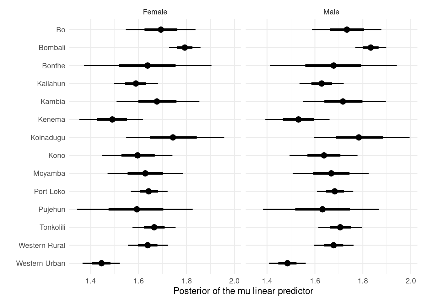
Figure 3.2: The posterior distribution of the linear predictor of mu parameter within the sex-district stratified model. The posterior expectations in Section 3.3 are a function of both the mu linear predictor posterior distribution and sigma linear predictor posterior distribution.

3.5 Delay posterior distributions

Posterior predictions of the delay distribution are an important output of an analysis with the epidist package. In this section, we demonstrate how to produce either a discrete probability mass function representation, or continuous probability density function representation of the delay distribution.

3.5.1 Discrete probability mass function

To generate a discrete probability mass function (PMF) we predict the delay distribution that would be observed with daily censoring and no right truncation. To do this, we set each of pwindow and swindow to 1 for daily censoring, and relative_obs_time to Inf for no right truncation. Figure 3.3 shows the result, where the few delays greater than 30 are omitted from the figure.

add_marginal_pmf_vars <- function(data) {
  data |>
    mutate(
      relative_obs_time = Inf, pwindow = 1, swindow = 1, delay_upr = NA
    )
}

draws_pmf <- obs_prep |>
  add_marginal_pmf_vars() |>
  add_predicted_draws(fit, ndraws = 1000)

pmf_base_figure <- ggplot(draws_pmf, aes(x = .prediction)) +
  geom_bar(aes(y = after_stat(count / sum(count)))) +
  labs(x = "", y = "", title = "Intercept-only", tag = "A") +
  scale_x_continuous(limits = c(0, 30)) +
  theme_minimal()

draws_sex_pmf <- obs_prep |>
  data_grid(sex) |>
  add_marginal_pmf_vars() |>
  add_predicted_draws(fit_sex, ndraws = 1000)

pmf_sex_figure <- draws_sex_pmf |>
  ggplot(aes(x = .prediction)) +
  geom_bar(aes(y = after_stat(
    count / ave(count, PANEL, FUN = sum)
  ))) +
  labs(x = "", y = "", title = "Sex-stratified", tag = "B") +
  facet_grid(. ~ sex) +
  scale_x_continuous(limits = c(0, 30)) +
  theme_minimal()

draws_sex_district_pmf <- obs_prep |>
  data_grid(sex, district) |>
  add_marginal_pmf_vars() |>
  add_predicted_draws(fit_sex_district, ndraws = 1000)

pmf_sex_district_figure <- draws_sex_district_pmf |>
  mutate(
    district = case_when(
      district == "Port Loko" ~ "Port\nLoko",
      district == "Western Rural" ~ "Western\nRural",
      district == "Western Urban" ~ "Western\nUrban",
      .default = district
    )
  ) |>
  ggplot(aes(x = .prediction)) +
  geom_bar(aes(y = after_stat(count / ave(count, PANEL, FUN = sum)))) +
  labs(
    x = "PMF with daily censoring and no truncation", y = "",
    title = "Sex-district-stratified", tag = "C"
  ) +
  facet_grid(district ~ sex) +
  scale_x_continuous(limits = c(0, 30)) +
  theme_minimal()

pmf_base_figure / pmf_sex_figure / pmf_sex_district_figure +
  plot_layout(heights = c(1, 1.5, 5.5))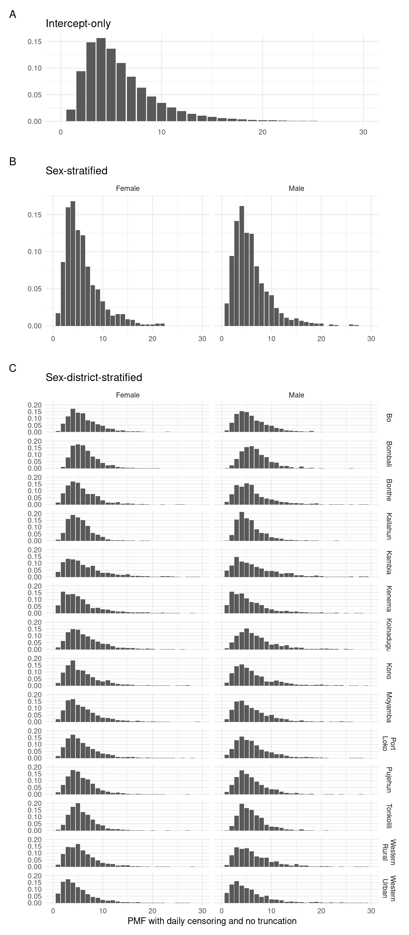

Figure 3.3: Posterior predictions of the discrete probability mass function for each of the fitted models.

3.5.2 Continuous probability density function

The posterior predictive distribution under no truncation and no censoring. That is to produce continuous delay times (Figure 3.4):

add_marginal_pdf_vars <- function(data) {
  data |>
    mutate(
      relative_obs_time = Inf, pwindow = 0, swindow = 0, delay_upr = NA
    )
}

draws_pdf <- obs_prep |>
  add_marginal_pdf_vars() |>
  add_predicted_draws(fit, ndraws = 1000)

pdf_base_figure <- ggplot(draws_pdf, aes(x = .prediction)) +
  geom_density() +
  labs(x = "", y = "", title = "Intercept-only", tag = "A") +
  scale_x_continuous(limits = c(0, 30)) +
  theme_minimal()

draws_sex_pdf <- obs_prep |>
  data_grid(sex) |>
  add_marginal_pdf_vars() |>
  add_predicted_draws(fit_sex, ndraws = 1000)

pdf_sex_figure <- draws_sex_pdf |>
  ggplot(aes(x = .prediction)) +
  geom_density() +
  labs(x = "", y = "", title = "Sex-stratified", tag = "B") +
  facet_grid(. ~ sex) +
  scale_x_continuous(limits = c(0, 30)) +
  theme_minimal()

draws_sex_district_pdf <- obs_prep |>
  data_grid(sex, district) |>
  add_marginal_pdf_vars() |>
  add_predicted_draws(fit_sex_district, ndraws = 1000)

pdf_sex_district_figure <- draws_sex_district_pdf |>
  mutate(
    district = case_when(
      district == "Port Loko" ~ "Port\nLoko",
      district == "Western Rural" ~ "Western\nRural",
      district == "Western Urban" ~ "Western\nUrban",
      .default = district
    )
  ) |>
  ggplot(aes(x = .prediction)) +
  geom_density() +
  labs(
    x = "PDF with no censoring and no truncation", y = "",
    title = "Sex-district-stratified", tag = "C"
  ) +
  facet_grid(district ~ sex) +
  scale_x_continuous(limits = c(0, 30)) +
  theme_minimal()

pdf_base_figure / pdf_sex_figure / pdf_sex_district_figure +
  plot_layout(heights = c(1, 1.5, 5.5))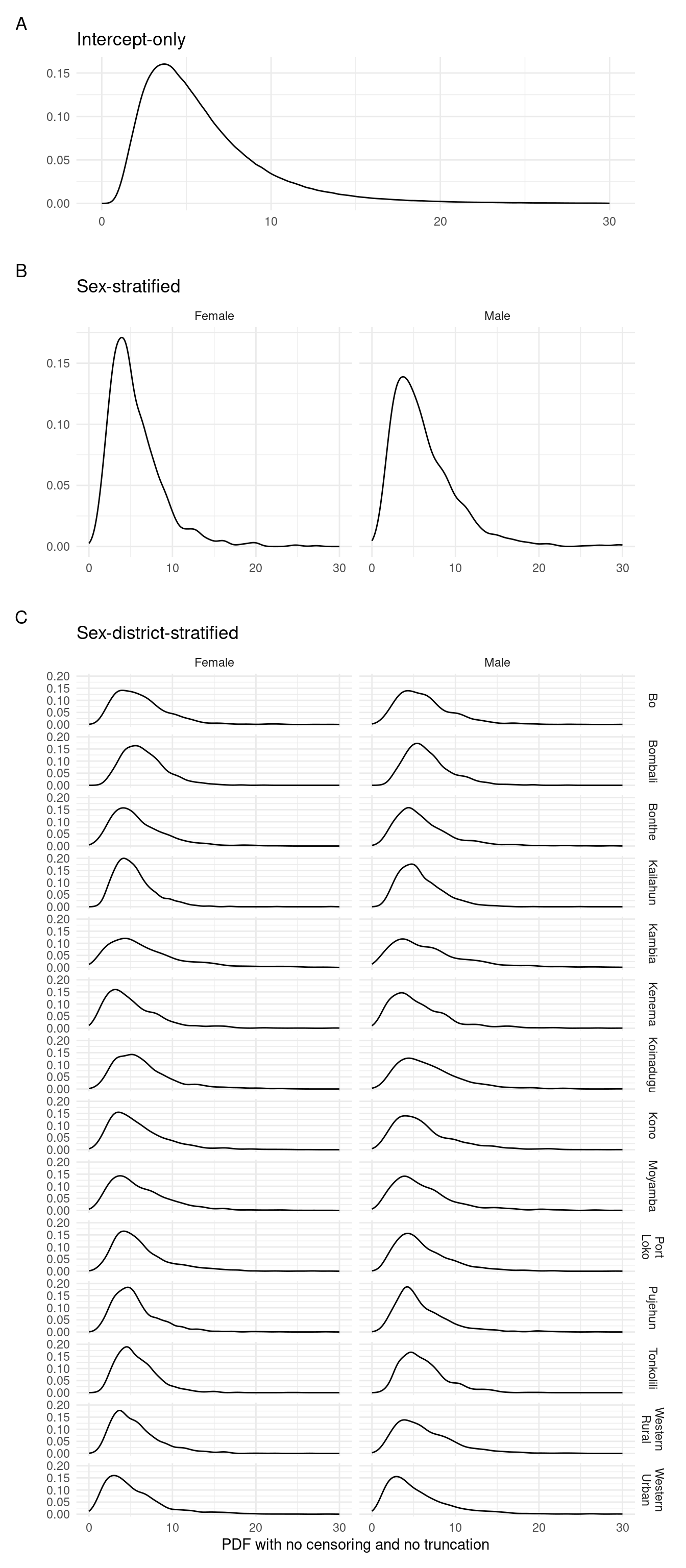

Figure 3.4: Posterior predictions of the continuous probability density function for each of the fitted models.

4 Conclusion

In this vignette, we demonstrate how the epidist package can be used to fit delay distribution models. These models can be stratified by covariates such as sex and district using fixed and random effects. Post-processing and prediction with fitted models is possible using the tidybayes package. We illustrate generating posterior expectations, the posteriors of linear predictors, as well as discrete and continuous representations of the delay distribution.

Bibliography

Fang, Li-Qun, Yang Yang, Jia-Fu Jiang, Hong-Wu Yao, David Kargbo, Xin-Lou Li, Bao-Gui Jiang, et al. 2016. “Transmission Dynamics of Ebola Virus Disease and Intervention Effectiveness in Sierra Leone.” Proceedings of the National Academy of Sciences 113 (16): 4488–93.

World Health Organization. 2016. “Ebola Outbreak 2014-2016 - West Africa.” https://www.who.int/emergencies/situations/ebola-outbreak-2014-2016-West-Africa.