Plot the observed delay distribution

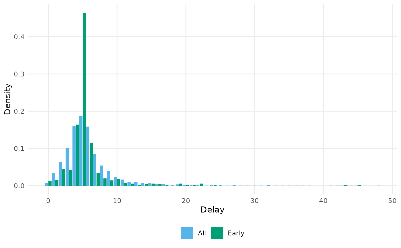
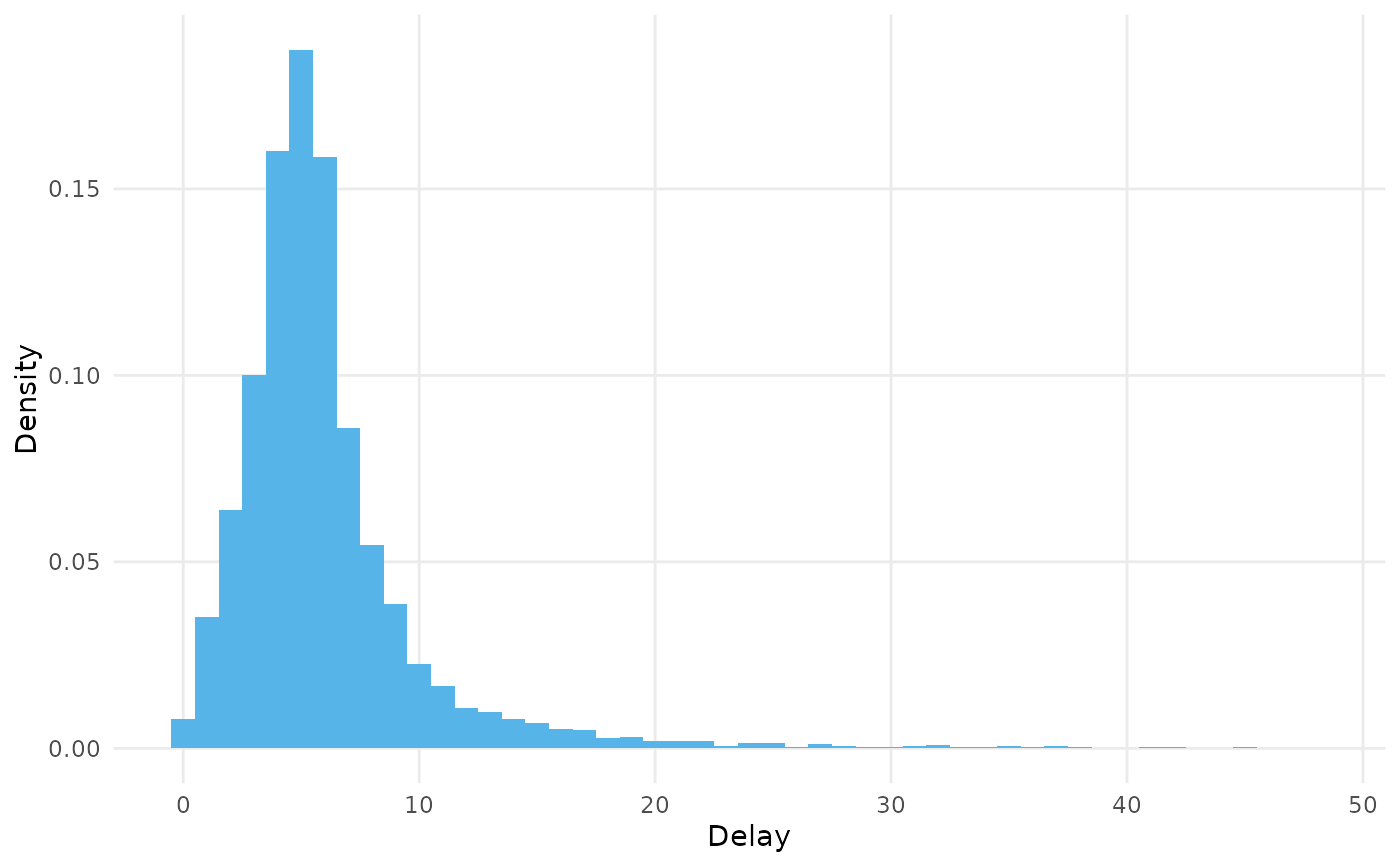
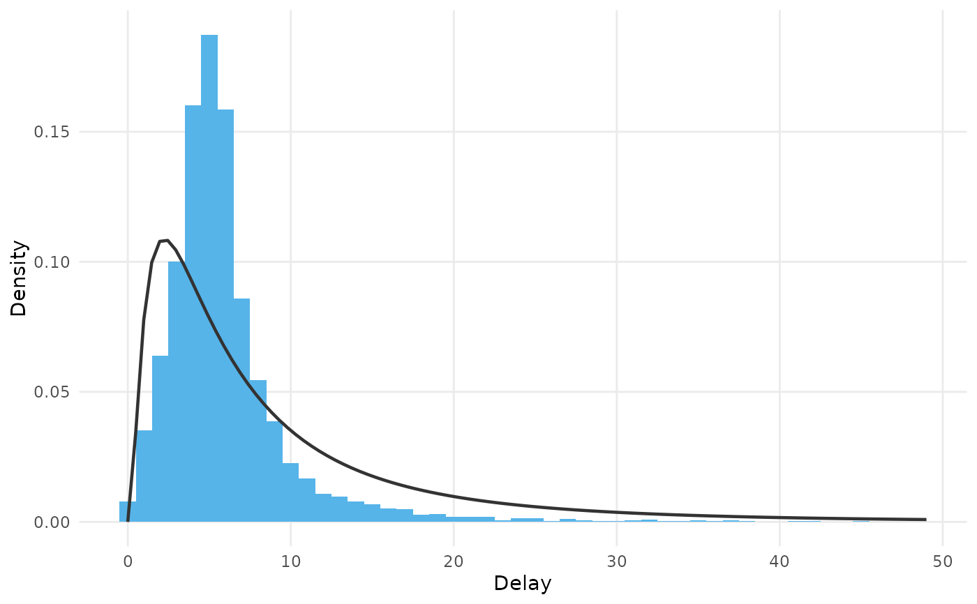
Bins the delay between the lower bounds of the primary and secondary event windows of each case, the delay as it was observed, and draws the proportion of cases in each bin as a column. Pass a named list of datasets to compare their observed delays, a reference distribution to draw the delay distribution they are a sample of, or a model fitted with epidist() to draw the delays it predicts over the delays it was fitted to.

Usage

plot_delays(x, ...)

Arguments

x

An epidist_linelist_data or epidist_aggregate_data object, a named list of them to compare, or a model fitted with epidist().

...

Passed to the method.

Value

A ggplot object.

Details

The observed delay is stime_lwr - ptime_lwr, the delay between the days the events were reported on when the data is censored daily. It is the response the naive model fits, so the plot shows the data that model sees rather than the delay distribution itself. Censoring and truncation both bias it, which is what the reference distribution makes visible.

Counts are weighted by the n column when the data has one, so aggregate data gives the same plot as the linelist it was aggregated from.

Proportions are within each stratum, so datasets of different sizes can be compared. The density is the proportion divided by binwidth, which puts the columns on the scale of the reference distribution.

The columns named by by are kept in the plot data, so the plot can be faceted by them.

See also

plot_events() to plot the event windows the delays come from, and plot.epidist_delay_draws() to plot a fitted delay distribution.

Other plot: plot.epidist_delay_draws(), plot_delays.default(), plot_delays.epidist_fit(), plot_delays.epidist_linelist_data(), plot_delays.list(), plot_events()

Examples

linelist <- sierra_leone_ebola_data |>
  as_epidist_linelist_data(
    pdate_lwr = "date_of_symptom_onset",
    sdate_lwr = "date_of_sample_tested"
  )
#> ℹ No primary event upper bound provided, using the primary event lower bound + 1 day as the assumed upper bound.
#> ℹ No secondary event upper bound provided, using the secondary event lower bound + 1 day as the assumed upper bound.
#> ℹ No observation time column provided, using 2015-09-14 as the observation date (the maximum of the secondary event upper bound).
plot_delays(linelist)

plot_delays(linelist, reference = c(mu = 1.8, sigma = 1))

plot_delays(list(All = linelist, Early = head(linelist, 500)))