1 Background
An event reported on a date could have happened at any point that day.
Models in epidist need an assumption about where, which we call the primary event distribution.
The default assumes it is equally likely at any point in the window. That holds when incidence is flat. It does not when incidence is growing or shrinking quickly. The event is then more likely towards one end of the window, and ignoring that biases the delay estimate (Charniga et al. 2024).
The primary event distributions come from primarycensored (Abbott et al. 2025).
vignette("model") gives the mathematical treatment.
2 Simulating from a growing epidemic
simulate_exponential_cases() draws primary events from an exponentially growing epidemic at rate r.
Here we use a rate of 0.5 and a lognormal delay.
Both events are censored to three day windows rather than daily ones.
Code
set.seed(101)

meanlog <- 1.6
sdlog <- 0.4
growth_rate <- 0.5
window <- 3

obs <- simulate_exponential_cases(r = growth_rate, sample_size = 500) |>
  simulate_secondary(meanlog = meanlog, sdlog = sdlog) |>
  simulate_dates(
    outbreak_start_date = as.Date("2024-01-01"), primary_window = window
  )

linelist <- as_epidist_linelist_data(obs)
plot_events() shows the windows each event is reported in.
Code
plot_events(linelist, n = 100)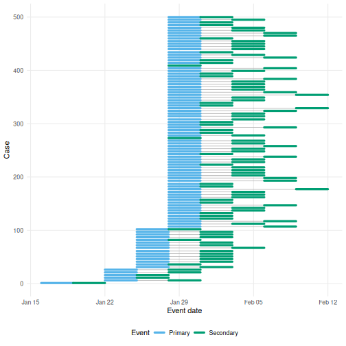
Figure 2.1: The event windows of 100 of the 500 simulated cases, ordered by primary event time. The primary windows are three days wide and the secondary windows one day.
3 Uniform against exponential growth
The marginal model takes the primary event distribution when the data are converted.
Code
uniform <- as_epidist_marginal_model(linelist, obs_time_threshold = 0)
growing <- as_epidist_marginal_model(
  linelist,
  primary = "expgrowth", obs_time_threshold = 0
)
With primary = "expgrowth" the growth rate becomes a distributional parameter called pgrowth.
It takes a formula and a prior in the same way as mu and sigma.
One set of delays carries little information about the growth rate, so here the prior does most of the work. Epidemic growth is normally estimated separately, from case counts over the same period. That estimate is then passed here as an informative prior centred on it, which is the approach taken in Brand et al. (2026). The prior below is centred on the rate used to simulate.
Code
The posterior for the rate stays close to the prior, which is expected.
Code
Both are compared against the delay used to simulate.
Code
uniform_draws <- delay_parameter_draws(fit_uniform)
growing_draws <- delay_parameter_draws(fit_growing)

draws <- bind_rows(
  Uniform = uniform_draws,
  `Exponential growth` = growing_draws,
  .id = "model"
) |>
  mutate(model = factor(model, levels = c("Uniform", "Exponential growth"))) |>
  add_summaries(family = fit_uniform)

plot(draws, by = "model", pars = "mu", true_values = c(mu = meanlog)) +
  labs(fill = "Primary event", colour = "Primary event")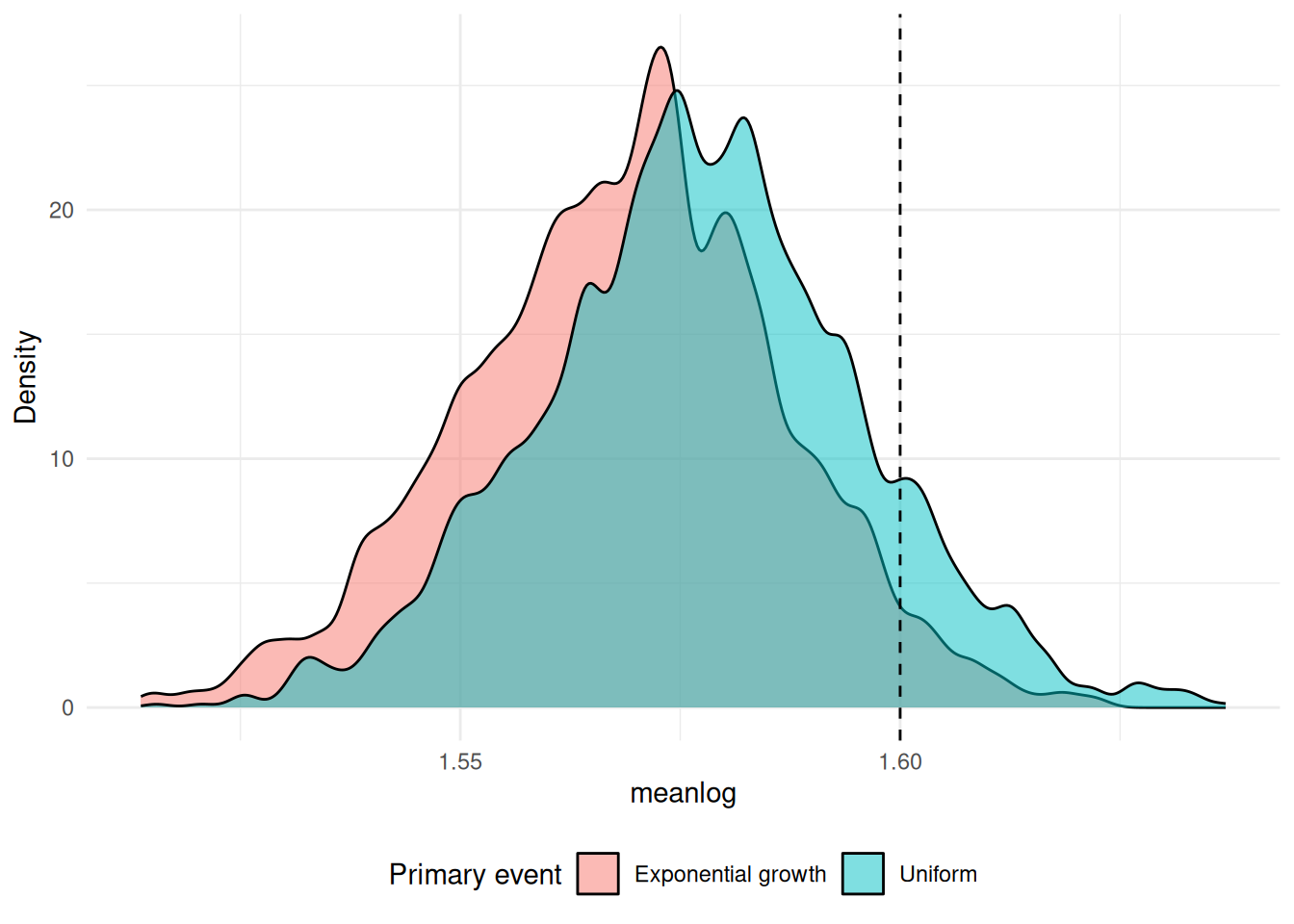
Figure 3.1: plot of chunk compare
4 A growth rate that varies
pgrowth takes a formula, so the rate can vary.
Here each location has its own rate, drawn around the shared value.
Each location is given its own seed, so they do not share random numbers.
Code
locations <- c(a = 0.2, b = 0.5, c = 0.8)

by_location <- purrr::imap(locations, function(r, location) {
  sim <- simulate_exponential_cases(
    r = r, sample_size = 300, seed = match(location, names(locations))
  ) |>
    simulate_secondary(meanlog = meanlog, sdlog = sdlog) |>
    simulate_dates(
      outbreak_start_date = as.Date("2024-01-01"), primary_window = window
    )
  return(mutate(sim, location = location))
})
by_location <- bind_rows(by_location)

linelist_locations <- as_epidist_linelist_data(by_location)
A random effect on pgrowth lets the rate differ by location while sharing information across them.
The marginal model is used here.
The latent model samples an event time per observation and would be slow at this size.
Code
marginal_locations <- as_epidist_marginal_model(
  linelist_locations,
  primary = "expgrowth",
  obs_time_threshold = 0
)

fit_locations <- epidist(
  marginal_locations,
  formula = bf(mu ~ 1, pgrowth ~ 1 + (1 | location)),
  prior = prior(normal(0.5, 0.2), class = "Intercept", dpar = "pgrowth") +
    prior(normal(0, 0.3), class = "sd", dpar = "pgrowth"),
  chains = 2, cores = 2, refresh = 0, silent = 2
)
Here the prior is shared across locations and the random effect lets each depart from it.
The prior on the standard deviation between locations is tight because three locations cannot tell you how much they vary.
Settings within one outbreak rarely differ in growth by more than a couple of tenths per day, which is the range normal(0, 0.3) allows.
Code
newdata <- epidist_newdata(marginal_locations, location = names(locations))

epred <- tidybayes::add_epred_draws(newdata, fit_locations, dpar = "pgrowth")

epred |>
  ggplot(aes(x = pgrowth, y = location)) +
  tidybayes::stat_halfeye(
    fill = "#56B4E9", colour = "#2A5674", .width = c(0.5, 0.95)
  ) +
  geom_point(
    data = tibble(location = names(locations), pgrowth = locations),
    colour = "#D55E00", size = 3
  ) +
  labs(x = "Growth rate", y = "Location") +
  theme_minimal()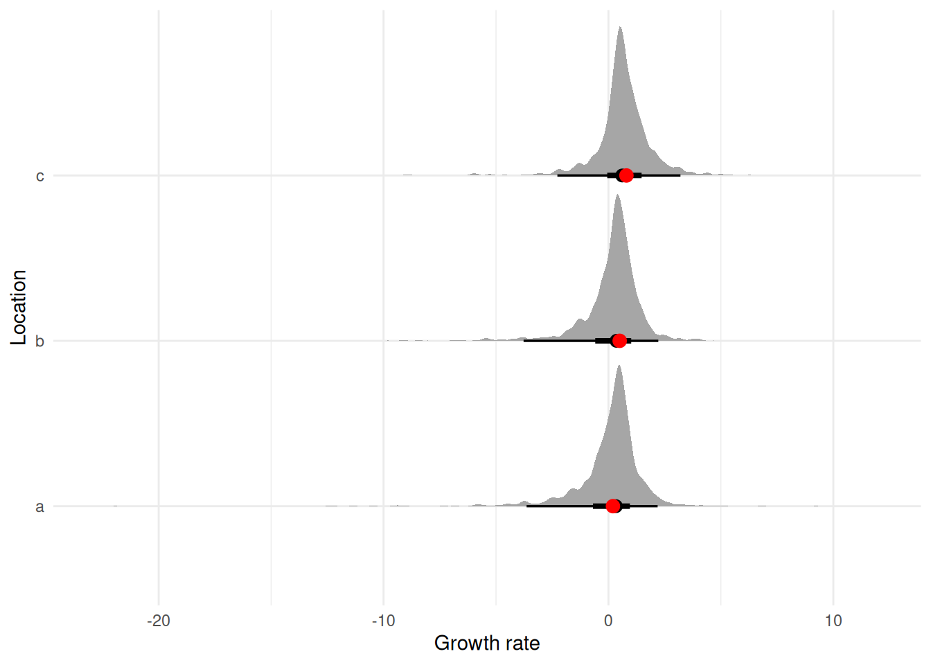
Figure 4.1: The posterior growth rate of each location. The points mark the rates the locations were simulated at.
4.1 Identifying the growth rate
A delay shared across locations cannot absorb a difference in growth between them, so the rates are better determined than they are from any one location alone. Refitting these data with a delay per location widens the interval on every rate by about a tenth. They are still far from pinned down, so an informative prior remains worth having.
5 Summary
- The distribution of the primary event within its window matters more the wider that window is, and the further the growth rate is from zero.
- Where the window is a day and the delay is several days, the default uniform assumption is usually enough. Weekly reporting, or fast growth or decline, is where it is not.
- Only the uniform and exponential growth distributions are supported. Others that are on the roadmap are a normal distribution, or a mixture of a normal distribution and a bounded exponential growth distribution.
- One set of delays carries little information about the growth rate, so take it from a separate estimate of epidemic growth and pass it as an informative prior.
- Several settings fitted together are a different matter. A delay shared across them cannot absorb a difference in growth between them, so the rates are better determined than they are from one setting alone.
- It would usually make sense to fit jointly with the case counts the growth rate would otherwise be estimated from, rather than passing a point estimate as a prior, but at the moment this requires a custom extension.
- Other uses of the primary event distribution are possible, such as a point source release where exposure is concentrated in a short window rather than spread across the reporting interval. These will usually need an informative prior on the delay distribution as well, since the data alone will not separate the two.